Hyperparameter Tuning Forecasts in Parallel with Modeltime
Written by Matt Dancho and Alberto González Almuiña
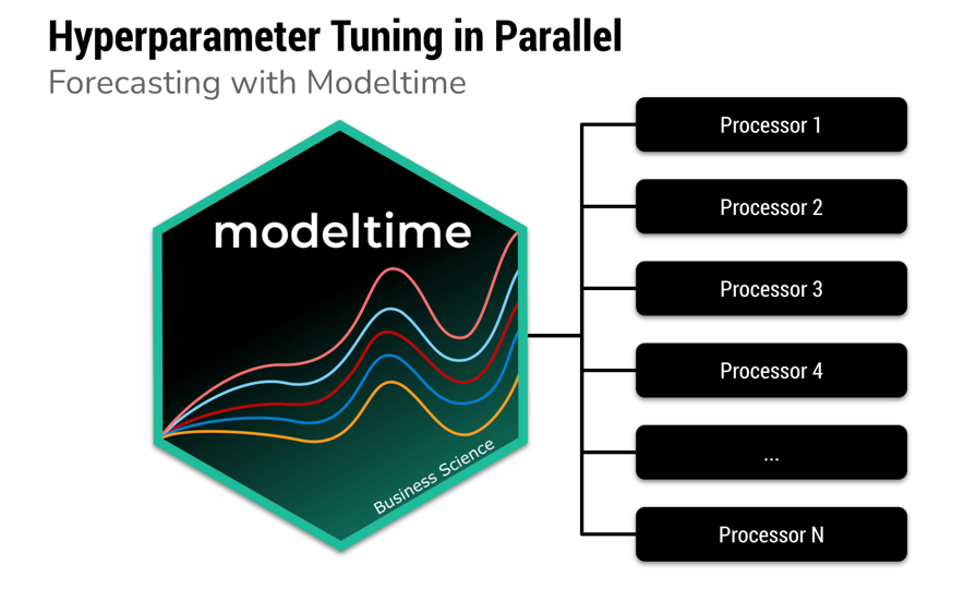
Speed up forecasting with modeltime’s new built-in parallel processing.
Fitting many time series models can be an expensive process. To help speed up computation, modeltime now includes parallel processing, which is support for high-performance computing by spreading the model fitting steps across multiple CPUs or clusters.
Highlights
-
We now have a new workflow for forecast model fitting with parallel processing that is much faster when creating many forecast models.
-
With 2-cores we got an immediate 30%-40% boost in performance. With more expensive processes and more CPU cores we get even more performance.
-
It’s perfect for hyperparameter tuning. See create_model_grid() for filling model specs with hyperparameters.
-
The workflow is simple. Just use parallel_start(6) to fire up 6-cores. Just use control_fit_workflowsets(allow_par = TRUE) to tell the modeltime_fit_workflowset() to run in parallel.
Forecast Hyperparameter Tuning Tutorial
Speed up forecasting
Speed up forecasting using multiple processors
In this tutorial, we go through a common Hyperparameter Tuning workflow that shows off the modeltime parallel processing integration and support for workflowsets from the tidymodels ecosystem. Hyperparameter tuning is an expensive process that can benefit from parallelization.
If you like what you see, I have an Advanced Time Series Course where you will learn the foundations of the growing Modeltime Ecosystem.
Time Series Forecasting Article Guide:
This article is part of a series of software announcements on the Modeltime Forecasting Ecosystem.
-
(Start Here) Modeltime: Tidy Time Series Forecasting using Tidymodels
-
Modeltime H2O: Forecasting with H2O AutoML
-
Modeltime Ensemble: Time Series Forecast Stacking
-
Modeltime Recursive: Tidy Autoregressive Forecasting
-
Hyperparameter Tuning Forecasts in Parallel with Modeltime
-
Time Series Forecasting Course: Now Available
Like these articles?
👉 Register to stay in the know
👈
on new cutting-edge R software like modeltime.
What is Modeltime?
A growing ecosystem for tidymodels forecasting
Modeltime is a growing ecosystem of forecasting packages used to develop scalable forecasting systems for your business.
The Modeltime Ecosystem extends tidymodels, which means any machine learning algorithm can now become a forecasting algorithm.
The Modeltime Ecosystem includes:
Out-of-the-Box
Parallel Processing Functionality Included
The newest feature of the modeltime package is parallel processing functionality. Modeltime comes with:
-
Use of parallel_start() and parallel_stop() to simplify the parallel processing setup.
-
Use of create_model_grid() to help generate parsnip model specs from dials parameter grids.
-
Use of modeltime_fit_workflowset() for initial fitting many models in parallel using workflowsets from the tidymodels ecosystem.
-
Use of modeltime_refit() to refit models in parallel.
-
Use of control_fit_workflowset() and control_refit() for controlling the fitting and refitting of many models.
Download the Cheat Sheet
As you go through this tutorial, it may help to use the Ultimate R Cheat Sheet. Page 3 covers the Modeltime Forecasting Ecosystem with links to key documentation.
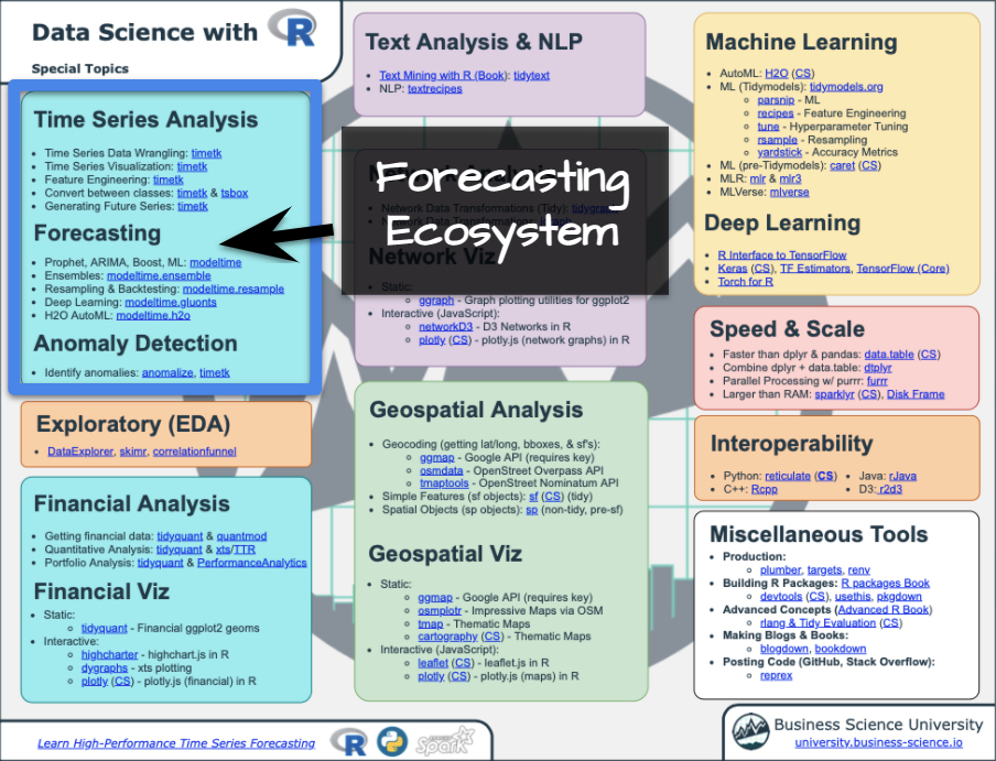
Forecasting Ecosystem Links (Ultimate R Cheat Sheet)
How to Use Parallel Processing
Let’s go through a common Hyperparameter Tuning workflow that shows off the modeltime parallel processing integration and support for workflowsets from the tidymodels ecosystem.
Libraries
Load the following libraries. Note that the new parallel processing functionality is available in Modeltime 0.6.1 (or greater).
# Machine Learning
library(modeltime) # Requires version >= 0.6.1
library(tidymodels)
library(workflowsets)

# Core
library(tidyverse)
library(timetk)
Setup Parallel Backend
I’ll set up this tutorial to use two (2) cores.
- To simplify creating clusters,
modeltime includes parallel_start(). We can simply supply the number of cores we’d like to use.
- To detect how many physical cores you have, you can run
parallel::detectCores(logical = FALSE).
parallel_start(2)
Load Data
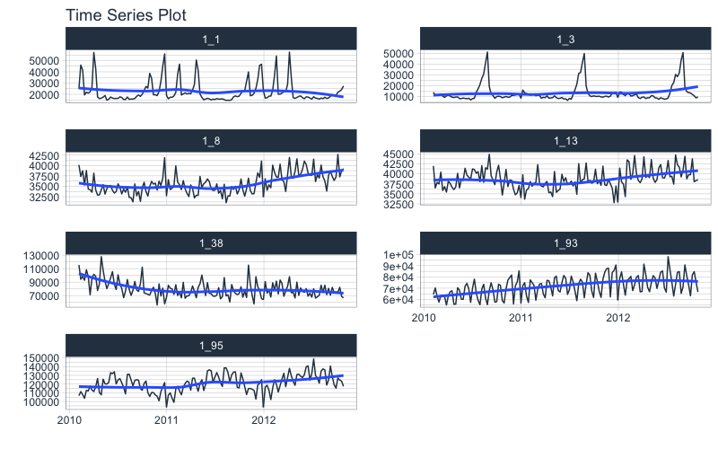
We’ll use the walmart_sales_weeekly dataset from timetk. It has seven (7) time series that represent weekly sales demand by department.
dataset_tbl <- walmart_sales_weekly %>%
  select(id, Date, Weekly_Sales)

dataset_tbl %>%
  group_by(id) %>%
  plot_time_series(
    .date_var    = Date,
    .value       = Weekly_Sales,
    .facet_ncol  = 2,
    .interactive = FALSE
  )
Train / Test Splits
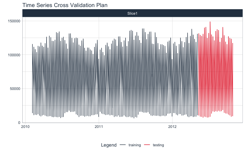
Use time_series_split() to make a temporal split for all seven time series.
splits <- time_series_split(
  dataset_tbl,
  assess     = "6 months",
  cumulative = TRUE
)

splits %>%
  tk_time_series_cv_plan() %>%
  plot_time_series_cv_plan(Date, Weekly_Sales, .interactive = F)
Recipe
Make a preprocessing recipe that generates time series features.
recipe_spec_1 <- recipe(Weekly_Sales ~ ., data = training(splits)) %>%
  step_timeseries_signature(Date) %>%
  step_rm(Date) %>%
  step_normalize(Date_index.num) %>%
  step_zv(all_predictors()) %>%
  step_dummy(all_nominal_predictors(), one_hot = TRUE)
Model Specifications
We’ll make 6 xgboost model specifications using boost_tree() and the “xgboost” engine. These will be combined with the recipe from the previous step using a workflow_set() in the next section.
The general idea
We can vary the learn_rate parameter to see it’s effect on forecast error.
# XGBOOST MODELS
model_spec_xgb_1 <- boost_tree(learn_rate = 0.001) %>%
  set_engine("xgboost")

model_spec_xgb_2 <- boost_tree(learn_rate = 0.010) %>%
  set_engine("xgboost")

model_spec_xgb_3 <- boost_tree(learn_rate = 0.100) %>%
  set_engine("xgboost")

model_spec_xgb_4 <- boost_tree(learn_rate = 0.350) %>%
  set_engine("xgboost")

model_spec_xgb_5 <- boost_tree(learn_rate = 0.500) %>%
  set_engine("xgboost")

model_spec_xgb_6 <- boost_tree(learn_rate = 0.650) %>%
  set_engine("xgboost")
A faster way
You may notice that this is a lot of repeated code to adjust the learn_rate. To simplify this process, we can use create_model_grid().
model_tbl <- tibble(
  learn_rate = c(0.001, 0.010, 0.100, 0.350, 0.500, 0.650)
) %>%
  create_model_grid(
    f_model_spec = boost_tree,
    engine_name  = "xgboost",
    mode         = "regression"
  )

model_tbl
## # A tibble: 6 x 2
##   learn_rate .models
##        <dbl> <list>
## 1      0.001 <spec[+]>
## 2      0.01  <spec[+]>
## 3      0.1   <spec[+]>
## 4      0.35  <spec[+]>
## 5      0.5   <spec[+]>
## 6      0.65  <spec[+]>
We can extract the model list for use with our workflowset next. This is the same result if we would have placed the manually generated 6 model specs into a list().
model_list <- model_tbl$.models

model_list
## [[1]]
## Boosted Tree Model Specification (regression)
##
## Main Arguments:
##   learn_rate = 0.001
##
## Computational engine: xgboost
##
##
## [[2]]
## Boosted Tree Model Specification (regression)
##
## Main Arguments:
##   learn_rate = 0.01
##
## Computational engine: xgboost
##
##
## [[3]]
## Boosted Tree Model Specification (regression)
##
## Main Arguments:
##   learn_rate = 0.1
##
## Computational engine: xgboost
##
##
## [[4]]
## Boosted Tree Model Specification (regression)
##
## Main Arguments:
##   learn_rate = 0.35
##
## Computational engine: xgboost
##
##
## [[5]]
## Boosted Tree Model Specification (regression)
##
## Main Arguments:
##   learn_rate = 0.5
##
## Computational engine: xgboost
##
##
## [[6]]
## Boosted Tree Model Specification (regression)
##
## Main Arguments:
##   learn_rate = 0.65
##
## Computational engine: xgboost
Workflowsets
With the workflow_set() function, we can combine the 6 xgboost models with the 1 recipe to return six (6) combinations of recipe and model specifications. These are currently untrained (unfitted).
model_wfset <- workflow_set(
  preproc = list(
    recipe_spec_1
  ),
  models = model_list,
  cross = TRUE
)

model_wfset
## # A workflow set/tibble: 6 x 4
##   wflow_id            info             option      result
##   <chr>               <list>           <list>      <list>
## 1 recipe_boost_tree_1 <tibble [1 × 4]> <wrkflw__ > <list [0]>
## 2 recipe_boost_tree_2 <tibble [1 × 4]> <wrkflw__ > <list [0]>
## 3 recipe_boost_tree_3 <tibble [1 × 4]> <wrkflw__ > <list [0]>
## 4 recipe_boost_tree_4 <tibble [1 × 4]> <wrkflw__ > <list [0]>
## 5 recipe_boost_tree_5 <tibble [1 × 4]> <wrkflw__ > <list [0]>
## 6 recipe_boost_tree_6 <tibble [1 × 4]> <wrkflw__ > <list [0]>
Parallel Training (Fitting)
We can train each of the combinations in parallel.
Controlling the Fitting Proces
Each fitting function in modeltime has a “control” function:
control_fit_workflowset() for modeltime_fit_workflowset()control_refit() for modeltime_refit()
The control functions help the user control the verbosity (adding remarks while training) and set up parallel processing. We can see the output when verbose = TRUE and allow_par = TRUE.
-
allow_par: Whether or not the user has indicated that parallel processing should be used.
-
If the user has set up parallel processing externally, the clusters will be reused.
-
If the user has not set up parallel processing, the fitting (training) process will set up parallel processing internally and shutdown. Note that this is more expensive, and usually costs around 10-15 seconds to set up.
-
verbose: Will return important messages showing the progress of the fitting operation.
-
cores: The cores that the user has set up. Since we’ve already set up doParallel to use 2 cores, the control recognizes this.
-
packages: The packages are packages that will be sent to each of the workers.
control_fit_workflowset(
  verbose   = TRUE,
  allow_par = TRUE
)
## workflowset control object
## --------------------------
## allow_par : TRUE
## cores     : 2
## verbose   : TRUE
## packages  : modeltime parsnip dplyr stats lubridate tidymodels timetk forcats stringr readr tidyverse yardstick workflowsets workflows tune tidyr tibble rsample recipes purrr modeldata infer ggplot2 dials scales broom graphics grDevices utils datasets methods base
Fitting Using Parallel Backend
We use the modeltime_fit_workflowset() and control_fit_workflowset() together to train the unfitted workflowset in parallel.
model_parallel_tbl <- model_wfset %>%
  modeltime_fit_workflowset(
    data    = training(splits),
    control = control_fit_workflowset(
      verbose   = TRUE,
      allow_par = TRUE
    )
  )
## Using existing parallel backend with 2 clusters (cores)...
##  Beginning Parallel Loop | 0.006 seconds
##  Finishing parallel backend. Clusters are remaining open. | 12.458 seconds
##  Close clusters by running: `parallel_stop()`.
##  Total time | 12.459 seconds
This returns a modeltime table.
model_parallel_tbl
## # Modeltime Table
## # A tibble: 6 x 3
##   .model_id .model     .model_desc
##       <int> <list>     <chr>
## 1         1 <workflow> XGBOOST
## 2         2 <workflow> XGBOOST
## 3         3 <workflow> XGBOOST
## 4         4 <workflow> XGBOOST
## 5         5 <workflow> XGBOOST
## 6         6 <workflow> XGBOOST
Comparison to Sequential Backend
We can compare to a sequential backend. We have a slight perfomance boost. Note that this performance benefit increases with the size of the training task.
model_sequential_tbl <- model_wfset %>%
  modeltime_fit_workflowset(
    data    = training(splits),
    control = control_fit_workflowset(
      verbose   = TRUE,
      allow_par = FALSE
    )
  )
## ℹ Fitting Model: 1
## ✓ Model Successfully Fitted: 1
## ℹ Fitting Model: 2
## ✓ Model Successfully Fitted: 2
## ℹ Fitting Model: 3
## ✓ Model Successfully Fitted: 3
## ℹ Fitting Model: 4
## ✓ Model Successfully Fitted: 4
## ℹ Fitting Model: 5
## ✓ Model Successfully Fitted: 5
## ℹ Fitting Model: 6
## ✓ Model Successfully Fitted: 6
## Total time | 15.781 seconds
Accuracy Assessment
We can review the forecast accuracy. We can see that Model 5 has the lowest MAE.
model_parallel_tbl %>%
  modeltime_calibrate(testing(splits)) %>%
  modeltime_accuracy() %>%
  table_modeltime_accuracy(.interactive = FALSE)
| .model_id |
.model_desc |
.type |
mae |
mape |
mase |
smape |
rmse |
rsq |
| 1 |
XGBOOST |
Test |
55572.50 |
98.52 |
1.63 |
194.17 |
66953.92 |
0.96 |
| 2 |
XGBOOST |
Test |
48819.23 |
86.15 |
1.43 |
151.49 |
58992.30 |
0.96 |
| 3 |
XGBOOST |
Test |
13426.89 |
21.69 |
0.39 |
25.06 |
17376.53 |
0.98 |
| 4 |
XGBOOST |
Test |
3699.94 |
8.94 |
0.11 |
8.68 |
5163.37 |
0.98 |
| 5 |
XGBOOST |
Test |
3296.74 |
7.30 |
0.10 |
7.37 |
5166.48 |
0.98 |
| 6 |
XGBOOST |
Test |
3612.70 |
8.15 |
0.11 |
8.24 |
5308.19 |
0.98 |
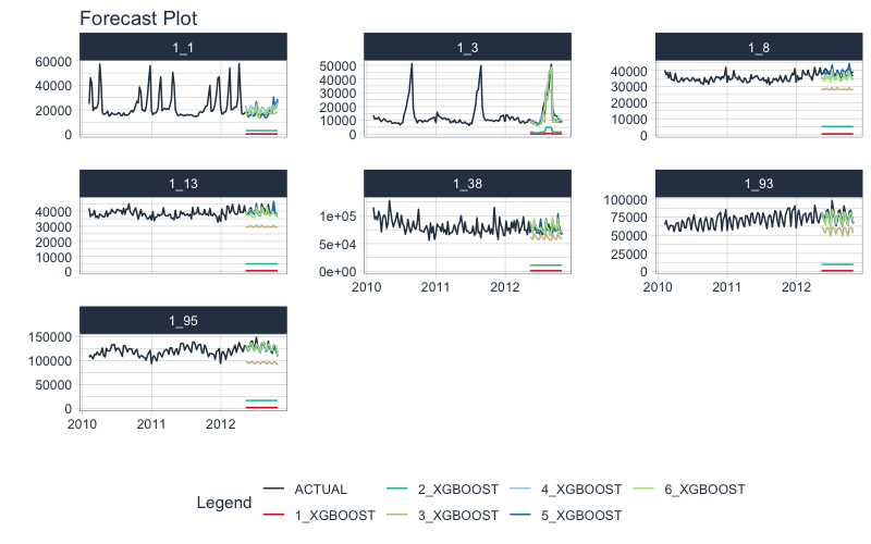
Forecast Assessment
We can visualize the forecast.
model_parallel_tbl %>%
  modeltime_forecast(
    new_data    = testing(splits),
    actual_data = dataset_tbl,
    keep_data   = TRUE
  ) %>%
  group_by(id) %>%
  plot_modeltime_forecast(
    .facet_ncol  = 3,
    .interactive = FALSE
  )
Closing Clusters
We can close the parallel clusters using parallel_stop().
parallel_stop()
It gets better
You’ve just scratched the surface, here’s what’s coming…
The Modeltime Ecosystem functionality is much more feature-rich than what we’ve covered here (I couldn’t possibly cover everything in this post). 😀
Here’s what I didn’t cover:
-
Feature Engineering: We can make this forecast much more accurate by including features from competition-winning strategies
-
Ensemble Modeling: We can stack H2O Models with other models not included in H2O like GluonTS Deep Learning.
-
Deep Learning: We can use GluonTS Deep Learning for developing high-performance, scalable forecasts.
So how are you ever going to learn time series analysis and forecasting?
You’re probably thinking:
- There’s so much to learn
- My time is precious
- I’ll never learn time series
I have good news that will put those doubts behind you.
You can learn time series analysis and forecasting in hours with my state-of-the-art time series forecasting course. 👇
High-Performance Time Series Course
Become the times series expert in your organization.
My High-Performance Time Series Forecasting in R course is available now. You’ll learn timetk and modeltime plus the most powerful time series forecasting techniques available like GluonTS Deep Learning. Become the times series domain expert in your organization.
👉 High-Performance Time Series Course.
You will learn:
- Time Series Foundations - Visualization, Preprocessing, Noise Reduction, & Anomaly Detection
- Feature Engineering using lagged variables & external regressors
- Hyperparameter Tuning - For both sequential and non-sequential models
- Time Series Cross-Validation (TSCV)
- Ensembling Multiple Machine Learning & Univariate Modeling Techniques (Competition Winner)
- Deep Learning with GluonTS (Competition Winner)
- and more.
Unlock the High-Performance Time Series Course
Project Roadmap, Future Work, and Contributing to Modeltime
Modeltime is a growing ecosystem of packages that work together for forecasting and time series analysis. Here are several useful links:
Acknowledgements
I’d like to acknowledge a Business Science University student that is part of the BSU Modeltime Dev Team. Alberto González Almuiña has helped BIG TIME with development of modeltime’s parallel processing functionality, contributing the initial software design. His effort is truly appreciated.
Have questions about Modeltime?
Make a comment in the chat below. 👇
And, if you plan on using modeltime for your business, it’s a no-brainer: Join my Time Series Course.