Introducing Modeltime Ensemble: Time Series Forecast Stacking
Written by Matt Dancho
I’m SUPER EXCITED to introduce modeltime.ensemble. Modeltime Ensemble implements three competition-winning forecasting strategies. This article (recently updated) introduces Modeltime Ensemble, which makes it easy to perform blended and stacked forecasts that improve forecast accuracy.
- We’ll quickly introduce you to the growing modeltime ecosystem.
- We’ll explain what Modeltime Ensemble does.
- Then, we’ll do a Modeltime Ensemble Forecast Tutorial using the
modeltime.ensemble
If you like what you see, I have an Advanced Time Series Course where you will become the time-series expert for your organization by learning modeltime, modeltime.ensemble, and timetk.
Time Series Forecasting Article Guide:
This article is part of a series of software announcements on the Modeltime Forecasting Ecosystem.
-
(Start Here) Modeltime: Tidy Time Series Forecasting using Tidymodels
-
Modeltime H2O: Forecasting with H2O AutoML
-
Modeltime Ensemble: Time Series Forecast Stacking
-
Modeltime Recursive: Tidy Autoregressive Forecasting
-
Hyperparameter Tuning Forecasts in Parallel with Modeltime
-
Time Series Forecasting Course: Now Available
Like these articles?
👉 Register to stay in the know
👈
on new cutting-edge R software like modeltime.
Meet the Modeltime Ecosystem
A growing ecosystem for tidymodels forecasting
Modeltime Ensemble is part of a growing ecosystem of Modeltime forecasting packages. The main purpose of the Modeltime Ecosystem is to develop scalable forecasting systems.
Modeltime Ensemble
The time series ensemble API for Modeltime
Three months ago I introduced modeltime, a new R package that speeds up forecasting experimentation and model selection with Machine Learning (XGBoost, GLMNET, Prophet, Prophet Boost, ARIMA, and ARIMA Boost). Fast-forward to now. I’m thrilled to announce the first expansion to the Modeltime Ecosystem: modeltime.ensemble.
Modeltime Ensemble is a cutting-edge package that integrates competition-winning time series ensembling strategies:
-
Stacked Meta-Learners
-
Weighted Ensembles
-
Average Ensembles
What is a Stacked Ensemble?
Using modeltime.ensemble, you can build something called a Stacked Ensemble. Let’s break this down:
-
An ensemble is just a combination of models. We can combine them in many ways.
-
One method is stacking, which typically uses a “meta-learning algorithm” to learn how to combine “sub-models” (the lower level models used as inputs to the stacking algorithm)
Stacking Diagram
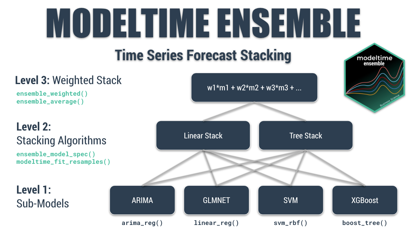
Here’s a Multi-Level Stack, which won the Kaggle Grupo Bimbo Inventory Demand Forecasting Competition.
The Multi-Level Stacked Ensemble that won the Kaggle Grupo Bimbo Inventory Demand Challenge
The multi-level stack can be broken down:
-
Level 1 - Sub-Models. Includes models like ARIMA, Elastic Net, Support Vector Machines, or XGBoost. These models each predict independently on the time series data.
-
Level 2 - Stacking Algorithms. Stacking algorithms learn how to combine each of the sub-models by training a “meta-model” on the predictions from the sub-models.
-
Level 3 - Weighted Stacking. Weighted stacking is a simple approach that is fast and effective. It’s a very simple approach where we apply a weighting and average the predictions of the incoming models. We can use this approach on sub-models, stacked models, or even a combination of stacked and sub-models. We decide the weighting.
I teach how to do a Multi-Level Stack in Module 14 of my High-Performance Time Series Forecasting Course.
What Modeltime Ensemble Functions do I need to know?
Here’s the low-down on which functions you’ll need to learn to implement different strategies. I teach these in in Module 14 of my High-Performance Time Series Forecasting Course.
-
Stacked Meta-Learners: Use modeltime_fit_resamples() to create sub-model predictions. Use ensemble_model_spec() to create super learners (models that learn from the predictions of sub-models).
-
Weighted Ensembles: Use ensemble_weighted() to create weighted ensemble blends. You choose the weights.
-
Average Ensembles: Use ensemble_average() to build simple average and median ensembles. No decisions necessary, but accuracy may be sub-optimal.
Ensemble Tutorial
Forecasting with Weighted Ensembles
Today, I’ll cover forecasting Product Sales Demand with Average and Weighted Ensembles, which are fast to implement and can have good performance (although stacked ensembles tend to have better performance).
Get the Cheat Sheet
As you go through this tutorial, it may help to use the Ultimate R Cheat Sheet. Page 3 Covers the Modeltime Forecasting Ecosystem with links to key documentation.
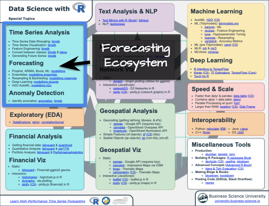
Forecasting Ecosystem Links (Ultimate R Cheat Sheet)
Modeltime Ensemble Diagram
Here’s an ensemble diagram of what we are going to accomplish.
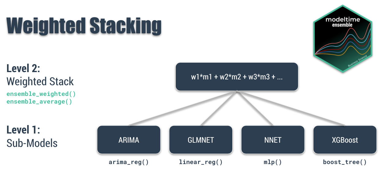
Weighted Stacking, Modeltime Ensemble Diagram
Modeltime Ensemble Functions used in this Tutorial
The idea is that we have several sub-models (Level 1) that make predictions. We can then take these predictions and blend them using weighting and averaging techniques (Level 2):
- Simple Average: Weights all models with the same proportion. Selects the average for each timestamp. Use
ensemble_average(type = "mean").
- Median Average: No weighting. Selects prediction using the centered value for each time stamp. Use
ensemble_average(type = "median").
- Weighted Average: User defines the weights (loadings). Applies a weighted average at each of the timestamps. Use
ensemble_weighted(loadings = c(1, 2, 3, 4)).
More Advanced Ensembles: Stacked Meta-Learners
The average and weighted ensembles are the simplest approaches to ensembling. One method that Modeltime Ensemble has integrated is Stacked Meta-Learners, which learn from the predictions of sub-models. We won’t cover stacked meta-learners in this tutorial. But, I teach them in my High-Performance Time Series Course. 💪
Getting Started
Let’s kick the tires on modeltime.ensemble
Install modeltime.ensemble.
install.packages("modeltime.ensemble")
Load the following libraries.
# Time Series Modeling and Machine Learning
library(tidymodels)
library(modeltime)
library(modeltime.ensemble)

# Time Series and Data Wrangling
library(timetk)
library(tidyverse)
Get Your Data
Forecasting Product Sales
Start with our Business Objective:
Our Business objective is to forecast the next 12-weeks of Product Sales Demandgiven 2-year sales history.
We’ll use the walmart_sales_weekly time series data set that includes Walmart Product Transactions from several stores, which is a small sample of the dataset from Kaggle Walmart Recruiting - Store Sales Forecasting. We’ll simplify the data set to a univariate time series with columns, “Date” and “Weekly_Sales” from Store 1 and Department 1.
store_1_1_tbl <- walmart_sales_weekly %>%
    filter(id == "1_1") %>%
    select(Date, Weekly_Sales)

store_1_1_tbl
## # A tibble: 143 x 2
##    Date       Weekly_Sales
##    <date>            <dbl>
##  1 2010-02-05       24924.
##  2 2010-02-12       46039.
##  3 2010-02-19       41596.
##  4 2010-02-26       19404.
##  5 2010-03-05       21828.
##  6 2010-03-12       21043.
##  7 2010-03-19       22137.
##  8 2010-03-26       26229.
##  9 2010-04-02       57258.
## 10 2010-04-09       42961.
## # … with 133 more rows
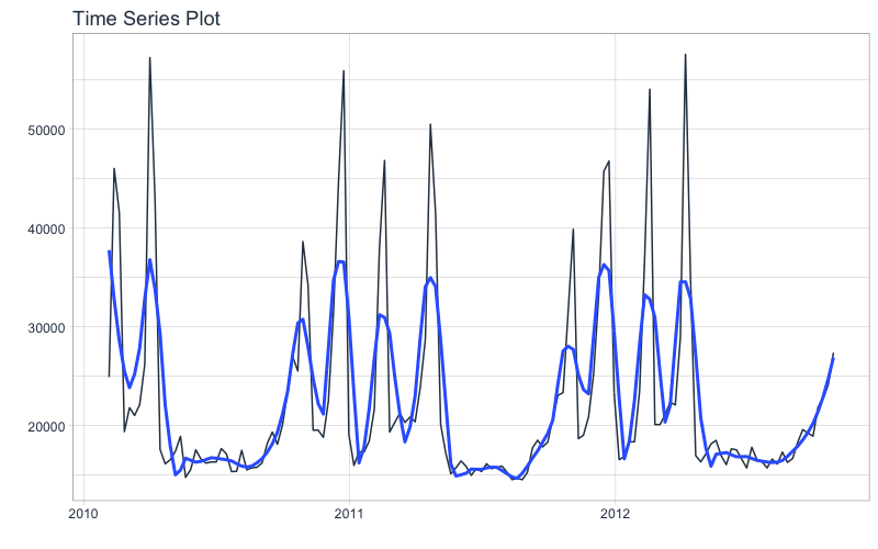
Next, visualize the dataset with the plot_time_series() function. Toggle .interactive = TRUE to get a plotly interactive plot. FALSE returns a ggplot2 static plot.
store_1_1_tbl %>%
    plot_time_series(Date, Weekly_Sales, .smooth_period = "3 months", .interactive = FALSE)
Seasonality Evaluation
Let’s do a quick seasonality evaluation to hone in on important features using plot_seasonal_diagnostics().
store_1_1_tbl %>%
    plot_seasonal_diagnostics(
        Date, Weekly_Sales,
        .feature_set = c("week", "month.lbl"),
        .interactive = FALSE
    )
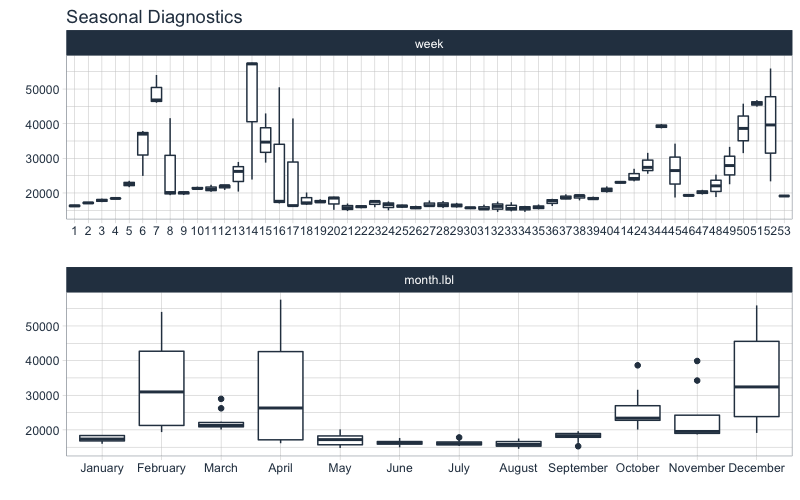
We can see that certain weeks and months of the year have higher sales. These anomalies are likely due to events. The Kaggle Competition informed competitors that Super Bowl, Labor Day, Thanksgiving, and Christmas were special holidays. To approximate the events, week number and month may be good features. Let’s come back to this when we preprocess our data.
Train / Test
Split your time series into training and testing sets
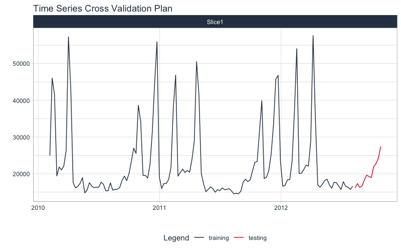
Give the objective to forecast 12 weeks of product sales, we use time_series_split() to make a train/test set consisting of 12-weeks of test data (hold out) and the rest for training.
- Setting
assess = "12 weeks" tells the function to use the last 12-weeks of data as the testing set.
- Setting
cumulative = TRUE tells the sampling to use all of the prior data as the training set.
splits <- store_1_1_tbl %>%
    time_series_split(assess = "12 weeks", cumulative = TRUE)
Next, visualize the train/test split.
tk_time_series_cv_plan(): Converts the splits object to a data frameplot_time_series_cv_plan(): Plots the time series sampling data using the “date” and “value” columns.
splits %>%
    tk_time_series_cv_plan() %>%
    plot_time_series_cv_plan(Date, Weekly_Sales, .interactive = FALSE)
Feature Engineering
We’ll make a number of calendar features using recipes. Most of the heavy lifting is done by timetk::step_timeseries_signature(), which generates a series of common time series features. We remove the ones that won’t help. After dummying we have 74 total columns, 72 of which are engineered calendar features.
recipe_spec <- recipe(Weekly_Sales ~ Date, store_1_1_tbl) %>%
    step_timeseries_signature(Date) %>%
    step_rm(matches("(iso$)|(xts$)|(day)|(hour)|(min)|(sec)|(am.pm)")) %>%
    step_mutate(Date_week = factor(Date_week, ordered = TRUE)) %>%
    step_dummy(all_nominal()) %>%
    step_normalize(contains("index.num"), Date_year)

recipe_spec %>% prep() %>% juice()
## # A tibble: 143 x 74
##    Date       Weekly_Sales Date_index.num Date_year Date_half Date_quarter
##    <date>            <dbl>          <dbl>     <dbl>     <int>        <int>
##  1 2010-02-05       24924.          -1.71     -1.21         1            1
##  2 2010-02-12       46039.          -1.69     -1.21         1            1
##  3 2010-02-19       41596.          -1.67     -1.21         1            1
##  4 2010-02-26       19404.          -1.64     -1.21         1            1
##  5 2010-03-05       21828.          -1.62     -1.21         1            1
##  6 2010-03-12       21043.          -1.59     -1.21         1            1
##  7 2010-03-19       22137.          -1.57     -1.21         1            1
##  8 2010-03-26       26229.          -1.54     -1.21         1            1
##  9 2010-04-02       57258.          -1.52     -1.21         1            2
## 10 2010-04-09       42961.          -1.50     -1.21         1            2
## # … with 133 more rows, and 68 more variables: Date_month <int>,
## #   Date_mweek <int>, Date_week2 <int>, Date_week3 <int>, Date_week4 <int>,
## #   Date_month.lbl_01 <dbl>, Date_month.lbl_02 <dbl>, Date_month.lbl_03 <dbl>,
## #   Date_month.lbl_04 <dbl>, Date_month.lbl_05 <dbl>, Date_month.lbl_06 <dbl>,
## #   Date_month.lbl_07 <dbl>, Date_month.lbl_08 <dbl>, Date_month.lbl_09 <dbl>,
## #   Date_month.lbl_10 <dbl>, Date_month.lbl_11 <dbl>, Date_week_01 <dbl>,
## #   Date_week_02 <dbl>, Date_week_03 <dbl>, Date_week_04 <dbl>,
## #   Date_week_05 <dbl>, Date_week_06 <dbl>, Date_week_07 <dbl>,
## #   Date_week_08 <dbl>, Date_week_09 <dbl>, Date_week_10 <dbl>,
## #   Date_week_11 <dbl>, Date_week_12 <dbl>, Date_week_13 <dbl>,
## #   Date_week_14 <dbl>, Date_week_15 <dbl>, Date_week_16 <dbl>,
## #   Date_week_17 <dbl>, Date_week_18 <dbl>, Date_week_19 <dbl>,
## #   Date_week_20 <dbl>, Date_week_21 <dbl>, Date_week_22 <dbl>,
## #   Date_week_23 <dbl>, Date_week_24 <dbl>, Date_week_25 <dbl>,
## #   Date_week_26 <dbl>, Date_week_27 <dbl>, Date_week_28 <dbl>,
## #   Date_week_29 <dbl>, Date_week_30 <dbl>, Date_week_31 <dbl>,
## #   Date_week_32 <dbl>, Date_week_33 <dbl>, Date_week_34 <dbl>,
## #   Date_week_35 <dbl>, Date_week_36 <dbl>, Date_week_37 <dbl>,
## #   Date_week_38 <dbl>, Date_week_39 <dbl>, Date_week_40 <dbl>,
## #   Date_week_41 <dbl>, Date_week_42 <dbl>, Date_week_43 <dbl>,
## #   Date_week_44 <dbl>, Date_week_45 <dbl>, Date_week_46 <dbl>,
## #   Date_week_47 <dbl>, Date_week_48 <dbl>, Date_week_49 <dbl>,
## #   Date_week_50 <dbl>, Date_week_51 <dbl>, Date_week_52 <dbl>
Make Sub-Models
Let’s make some sub-models with Modeltime
Now for the fun part! Let’s make some models using functions from modeltime and parsnip.
Auto ARIMA
Here’s the basic Auto ARIMA Model.
- Model Spec:
arima_reg() <– This sets up your general model algorithm and key parameters
- Set Engine:
set_engine("auto_arima") <– This selects the specific package-function to use and you can add any function-level arguments here.
- Fit Model:
fit(Weekly_Sales ~ Date, training(splits)) <– All Modeltime Models require a date column to be a regressor.
model_fit_arima <- arima_reg(seasonal_period = 52) %>%
    set_engine("auto_arima") %>%
    fit(Weekly_Sales ~ Date, training(splits))

model_fit_arima
## parsnip model object
##
## Fit time:  206ms
## Series: outcome
## ARIMA(0,0,1)(0,1,0)[52]
##
## Coefficients:
##          ma1
##       0.6704
## s.e.  0.0767
##
## sigma^2 estimated as 60063672:  log likelihood=-819.37
## AIC=1642.74   AICc=1642.9   BIC=1647.48
Elastic Net
Making an Elastic NET model is easy to do. Just set up your model spec using linear_reg() and set_engine("glmnet"). Note that we have not fitted the model yet (as we did in previous steps).
model_spec_glmnet <- linear_reg(penalty = 0.01, mixture = 0.5) %>%
    set_engine("glmnet")
Next, make a fitted workflow:
- Start with a
workflow()
- Add a Model Spec:
add_model(model_spec_glmnet)
- Add Preprocessing:
add_recipe(recipe_spec %>% step_rm(date)) <– Note that I’m removing the “date” column since Machine Learning algorithms don’t typically know how to deal with date or date-time features
- Fit the Workflow:
fit(training(splits))
wflw_fit_glmnet <- workflow() %>%
    add_model(model_spec_glmnet) %>%
    add_recipe(recipe_spec %>% step_rm(Date)) %>%
    fit(training(splits))
XGBoost
We can fit a XGBoost Model using a similar process as the Elastic Net.
model_spec_xgboost <- boost_tree() %>%
    set_engine("xgboost")

set.seed(123)
wflw_fit_xgboost <- workflow() %>%
    add_model(model_spec_xgboost) %>%
    add_recipe(recipe_spec %>% step_rm(Date)) %>%
    fit(training(splits))
NNETAR
We can use a NNETAR model. Note that add_recipe() uses the full recipe (with the Date column) because this is a Modeltime Model.
model_spec_nnetar <- nnetar_reg(
        seasonal_period = 52,
        non_seasonal_ar = 4,
        seasonal_ar     = 1
    ) %>%
    set_engine("nnetar")

set.seed(123)
wflw_fit_nnetar <- workflow() %>%
    add_model(model_spec_nnetar) %>%
    add_recipe(recipe_spec) %>%
    fit(training(splits))
Prophet w/ Regressors
We’ll build a Prophet Model with Regressors. This uses the Facebook Prophet forecasting algorithm and supplies all of the 72 features as regressors to the model. Note - Because this is a Modeltime Model we need to have a Date Feature in the recipe.
model_spec_prophet <- prophet_reg(
      seasonality_yearly = TRUE
    ) %>%
    set_engine("prophet")

wflw_fit_prophet <- workflow() %>%
    add_model(model_spec_prophet) %>%
    add_recipe(recipe_spec) %>%
    fit(training(splits))
Sub-Model Evaluation
Let’s take a look at our progress so far. We have 5 models. We’ll put them into a Modeltime Table to organize them using modeltime_table().
submodels_tbl <- modeltime_table(
    model_fit_arima,
    wflw_fit_glmnet,
    wflw_fit_xgboost,
    wflw_fit_nnetar,
    wflw_fit_prophet
)

submodels_tbl
## # Modeltime Table
## # A tibble: 5 x 3
##   .model_id .model     .model_desc
##       <int> <list>     <chr>
## 1         1 <fit[+]>   ARIMA(0,0,1)(0,1,0)[52]
## 2         2 <workflow> GLMNET
## 3         3 <workflow> XGBOOST
## 4         4 <workflow> NNAR(4,1,10)[52]
## 5         5 <workflow> PROPHET W/ REGRESSORS
We can get the accuracy on the hold-out set using modeltime_accuracy() and table_modeltime_accuracy(). The best model is the Prophet with Regressors with a MAE of 1031.
submodels_tbl %>%
    modeltime_accuracy(testing(splits)) %>%
    table_modeltime_accuracy(.interactive = FALSE)
| .model_id |
.model_desc |
.type |
mae |
mape |
mase |
smape |
rmse |
rsq |
| 1 |
ARIMA(0,0,1)(0,1,0)[52] |
Test |
1359.99 |
6.77 |
1.02 |
6.93 |
1721.47 |
0.95 |
| 2 |
GLMNET |
Test |
1222.38 |
6.47 |
0.91 |
6.73 |
1349.88 |
0.98 |
| 3 |
XGBOOST |
Test |
1089.56 |
5.22 |
0.82 |
5.20 |
1266.62 |
0.96 |
| 4 |
NNAR(4,1,10)[52] |
Test |
2529.92 |
11.68 |
1.89 |
10.73 |
3507.55 |
0.93 |
| 5 |
PROPHET W/ REGRESSORS |
Test |
1031.53 |
5.13 |
0.77 |
5.22 |
1226.80 |
0.98 |
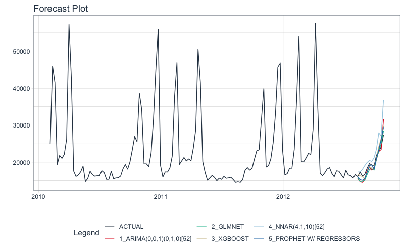
And, we can visualize the forecasts with modeltime_forecast() and plot_modeltime_forecast().
submodels_tbl %>%
    modeltime_forecast(
        new_data    = testing(splits),
        actual_data = store_1_1_tbl
    ) %>%
    plot_modeltime_forecast(.interactive = FALSE)
Build Modeltime Ensembles
This is exciting.
We’ll make Average, Median, and Weighted Ensembles. If you are interested in making Super Learners (Meta-Learner Models that leverage sub-model predictions), I teach this in my new High-Performance Time Series course.
I’ve made it super simple to build an ensemble from a Modeltime Tables. Here’s how to use ensemble_average().
- Start with your Modeltime Table of Sub-Models
- Pipe into
ensemble_average(type = "mean")
You now have a fitted average ensemble.
# Simple Average Ensemble
ensemble_fit_avg <- submodels_tbl %>%
    ensemble_average(type = "mean")

ensemble_fit_avg
## ── Modeltime Ensemble ───────────────────────────────────────────
## Ensemble of 5 Models (MEAN)
##
## # Modeltime Table
## # A tibble: 5 x 3
##   .model_id .model     .model_desc
##       <int> <list>     <chr>
## 1         1 <fit[+]>   ARIMA(0,0,1)(0,1,0)[52]
## 2         2 <workflow> GLMNET
## 3         3 <workflow> XGBOOST
## 4         4 <workflow> NNAR(4,1,10)[52]
## 5         5 <workflow> PROPHET W/ REGRESSORS
We can make median and weighted ensembles just as easily. Note - For the weighted ensemble I’m loading the better performing models higher.
# Simple Median Ensemble
ensemble_fit_med <- submodels_tbl %>%
    ensemble_average("median")

# Higher Loading on Better Models (Test RMSE)
ensemble_fit_wt <- submodels_tbl %>%
    ensemble_weighted(loadings = c(2, 4, 6, 1, 6))
Ensemble Evaluation
Let’s see how we did
We need to have Modeltime Tables that organize our ensembles before we can assess performance. Just use modeltime_table() to organize ensembles just like we did for the Sub-Models.
ensemble_models_tbl <- modeltime_table(
    ensemble_fit_avg,
    ensemble_fit_med,
    ensemble_fit_wt
)

ensemble_models_tbl
## # Modeltime Table
## # A tibble: 3 x 3
##   .model_id .model         .model_desc
##       <int> <list>         <chr>
## 1         1 <ensemble [5]> ENSEMBLE (MEAN): 5 MODELS
## 2         2 <ensemble [5]> ENSEMBLE (MEDIAN): 5 MODELS
## 3         3 <ensemble [5]> ENSEMBLE (WEIGHTED): 5 MODELS
Let’s check out the Accuracy Table using modeltime_accuracy() and table_modeltime_accuracy().
- From MAE, Ensemble Model ID 1 has 1000 MAE, a 3% improvement over our best submodel (MAE 1031).
- From RMSE, Ensemble Model ID 3 has 1228, which is on par with our best submodel.
ensemble_models_tbl %>%
    modeltime_accuracy(testing(splits)) %>%
    table_modeltime_accuracy(.interactive = FALSE)
| .model_id |
.model_desc |
.type |
mae |
mape |
mase |
smape |
rmse |
rsq |
| 1 |
ENSEMBLE (MEAN): 5 MODELS |
Test |
1000.01 |
4.63 |
0.75 |
4.58 |
1408.68 |
0.97 |
| 2 |
ENSEMBLE (MEDIAN): 5 MODELS |
Test |
1146.60 |
5.68 |
0.86 |
5.77 |
1310.30 |
0.98 |
| 3 |
ENSEMBLE (WEIGHTED): 5 MODELS |
Test |
1056.59 |
5.15 |
0.79 |
5.20 |
1228.45 |
0.98 |
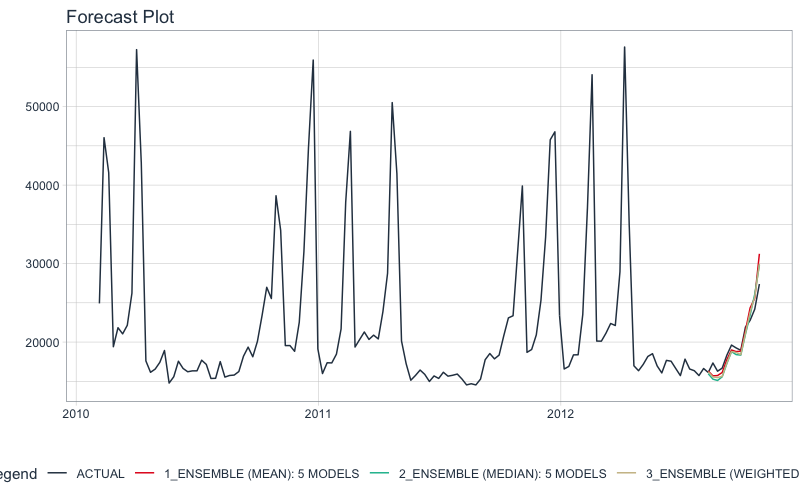
And finally we can visualize the performance of the ensembles.
ensemble_models_tbl %>%
    modeltime_forecast(
        new_data    = testing(splits),
        actual_data = store_1_1_tbl
    ) %>%
    plot_modeltime_forecast(.interactive = FALSE)
It gets better
You’ve just scratched the surface, here’s what’s coming…
The modeltime.ensemble package functionality is much more feature-rich than what we’ve covered here (I couldn’t possibly cover everything in this post). 😀
Here’s what I didn’t cover:
-
Scalable Forecasting with Ensembles: What happens when your data has more than one time series. This is called scalable forecasting, and we need to use special techniques to ensemble these models.
-
Stacked Super-Learners: We can make use resample predictions from our sub-models as inputs to a meta-learner. This can result is significantly better accuracy (5% improvement is what we achieve in my Time Series Course).
-
Multi-Level Stacking: This is the strategy that won the Grupo Bimbo Inventory Demand Forecasting Challenge where multiple layers of ensembles are used.
-
Refitting Sub-Models and Meta-Learners: Refitting is special task that is needed prior to forecasting future data. Refitting requires careful attention to control the sub-model and meta-learner retraining process.
So how are you ever going to learn time series analysis and forecasting?
You’re probably thinking:
- There’s so much to learn
- My time is precious
- I’ll never learn time series
I have good news that will put those doubts behind you.
You can learn time series analysis and forecasting in hours with my state-of-the-art time series forecasting course. 👇
High-Performance Time Series Course
Become the times series expert in your organization.
My High-Performance Time Series Forecasting in R course is available now. You’ll learn timetk and modeltime plus the most powerful time series forecasting techniques available like GluonTS Deep Learning. Become the times series domain expert in your organization.
👉 High-Performance Time Series Course.
You will learn:
- Time Series Foundations - Visualization, Preprocessing, Noise Reduction, & Anomaly Detection
- Feature Engineering using lagged variables & external regressors
- Hyperparameter Tuning - For both sequential and non-sequential models
- Time Series Cross-Validation (TSCV)
- Ensembling Multiple Machine Learning & Univariate Modeling Techniques (Competition Winner)
- Deep Learning with GluonTS (Competition Winner)
- and more.
Unlock the High-Performance Time Series Course
Project Roadmap, Future Work, and Contributing to Modeltime
Modeltime is a growing ecosystem of packages that work together for forecasting and time series analysis. Here are several useful links:
Have questions about Modeltime Ensemble?
Make a comment in the chat below. 👇
And, if you plan on using modeltime.ensemble for your business, it’s a no-brainer - Take my Time Series Course.