Introducing Modeltime Recursive: Tidy Autoregressive Forecasting with Lags
Written by Matt Dancho and Alberto González Almuiña
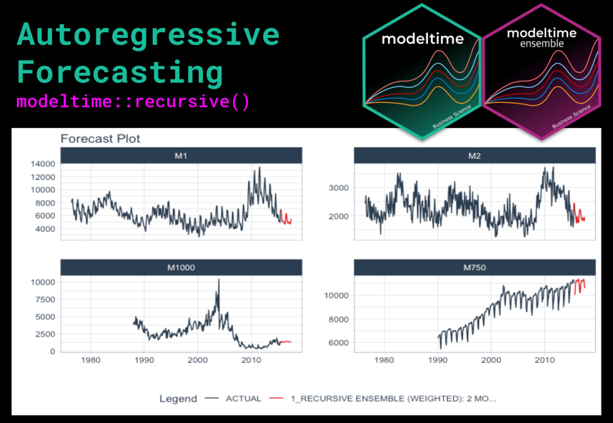
I’m super excited to introduce modeltime::recursive(), the new autoregressive forecast solution that allows you to convert any tidymodels regression algorithm into an autoregressive forecasting algorithm. Think of Recursive as a Lag Management Tool.
The new Autoregressive Machine Learning (AR-ML) Forecasting Solution handles lags for one or more time series and was just greatly improved in Modeltime 0.5.0 (just released 🎉). This Tidy Forecasting Tutorial introduces modeltime::recursive(): our new Tidy Autoregressive Forecast Solution.
If you like what you see, I have an Advanced Time Series Course where you will learn the foundations of the growing Modeltime Ecosystem.
Time Series Forecasting Article Guide:
This article is part of a series of software announcements on the Modeltime Forecasting Ecosystem.
-
(Start Here) Modeltime: Tidy Time Series Forecasting using Tidymodels
-
Modeltime H2O: Forecasting with H2O AutoML
-
Modeltime Ensemble: Time Series Forecast Stacking
-
Modeltime Recursive: Tidy Autoregressive Forecasting
-
Hyperparameter Tuning Forecasts in Parallel with Modeltime
-
Time Series Forecasting Course: Now Available
Like these articles?
👉 Register to stay in the know
👈
on new cutting-edge R software like modeltime.
The Problem with Autoregressive Forecasting: Lags make Missing Values
Forecasting with autoregressive features is a challenge. The problem is that Lags make missing values that show up as NA.
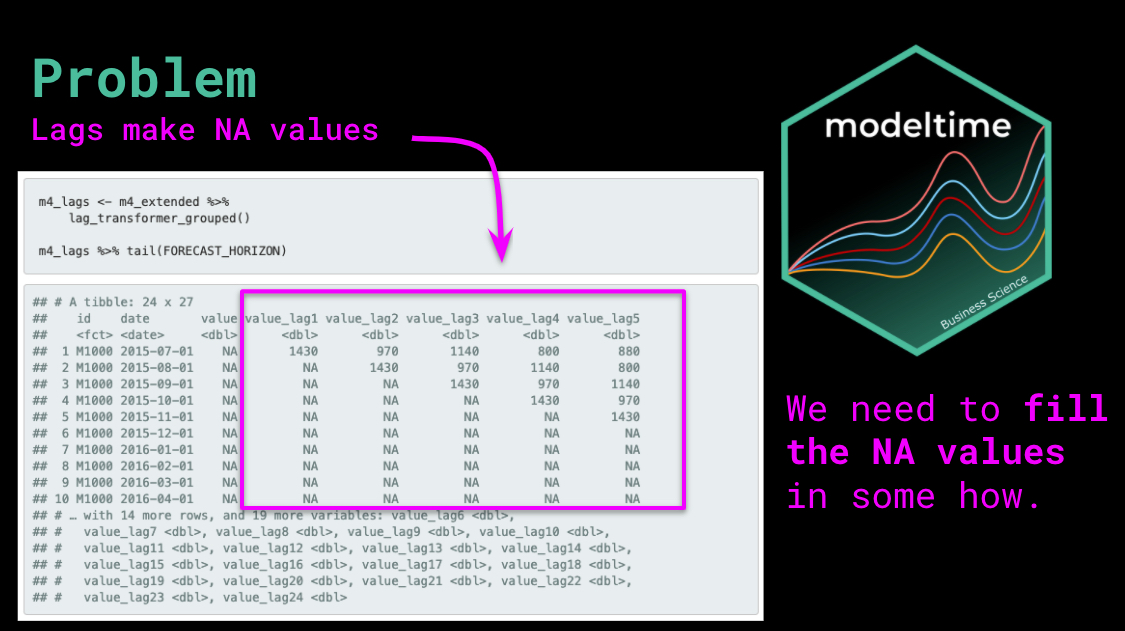
This isn’t a new problem. Algorithms like ARIMA have been managing this internally for one time series at a time for decades. But, they’ve only been doing it for one time series at a time forcing us to loop through every time series for prediction. This iterative approach is not scalable with modern machine learning.
The new challenge is how do we manage this for multiple time series? If you have more than one time series, this quickly becomes a forecasting nightmare that will make your head spin. Then multiply this by the number of different modeling algorithms you want to experiment with, and, well, you get the picture…
Enter modeltime::recursive(): A new function that is capable of turning any Tidymodels regression algorithm into an autoregressive forecaster.
It’s a Lag Management Tool that handles the lagged predictions on one or more time series.
Solution: modeltime::recursive()
Autoregressive forecasting with lag management.
Modeltime 0.5.0 includes a new and improved modeltime::recursive() function that turns any tidymodels regression algorithm into an autoregressive forecaster.
✅ Hassle-Free
Recursive is a new way to manage lagged regressors used in autoregressive forecasting.
✅ Any Tidymodel can become Autoregressive.
Recursive can be used with any regression model that is part of the tidymodels ecosystem (e.g. XGBoost, Random Forest, GLMNET).
✅ Works with Multiple Time Series.
Recursive works on single time series and multiple time series (panel data).
✅ Works with Ensembles.
Recursive can also be used in Ensembles (Recursive Ensembles) with modeltime.ensemble 0.4.0 (just released, yay! 🎉).
What do you need to do to get Recursive?
Simply upgrade to modeltime and modeltime.ensemble. Both were just released to CRAN.
install.packages(c('modeltime', 'modeltime.ensemble'))
This version of the tutorial uses the “development version” of both packages. We are improving this software a lot as we grow the Modeltime Ecosystem. If you’d like to install the development version with the latest features:
remotes::install_github("business-science/modeltime")
remotes::install_github("business-science/modeltime.ensemble")
Autoregressive Forecast Tutorial
Combine recursive() with Modeltime Ensemble
Here’s what we’re making:
- A Recursive Ensemble with
modeltime.ensemble 0.4.0
- That uses two sub-models: 40% GLMNET and 60% XGBOOST
- With Lags 1-24 as the main features using
modeltime::recursive() to manage the process
- We will forecast 24 months (2-years) using lags < forecast horizon
Get the Cheat Sheet
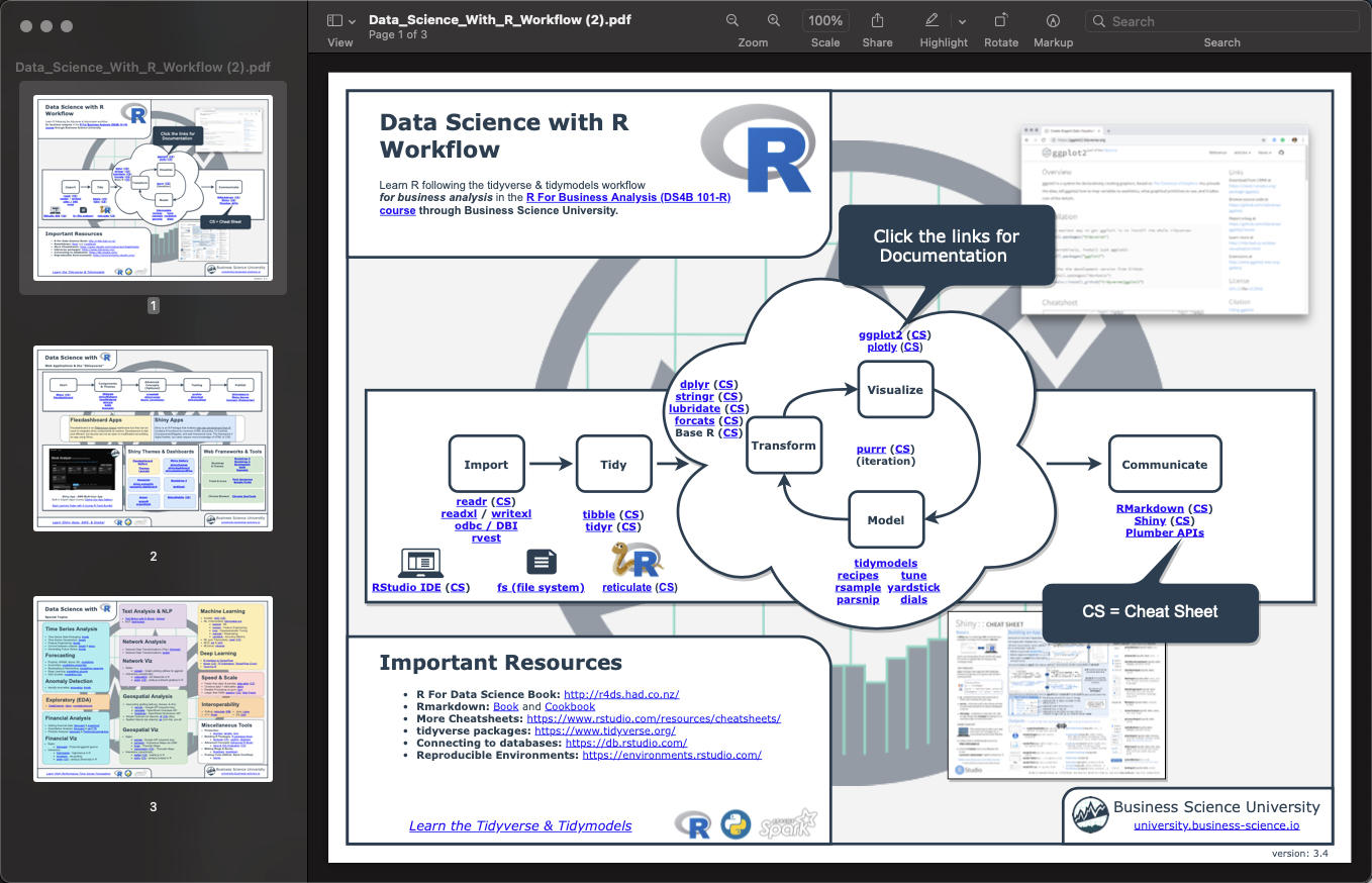
As you go through this tutorial, you will see many references to the Ultimate R Cheat Sheet. The Ultimate R Cheatsheet covers the Modeltime Forecasting Ecosystem with links to key documentation. You can download the Ultimate R Cheat Sheet for free.
Download the Ultimate R Cheat Sheet (Free)
We’ll be focusing on three key packages: timetk, modeltime and modeltime.ensemble. Links to the documentation are included in the cheat sheet (every package has a hyperlink, and some even have “CS” links to their cheat sheets).
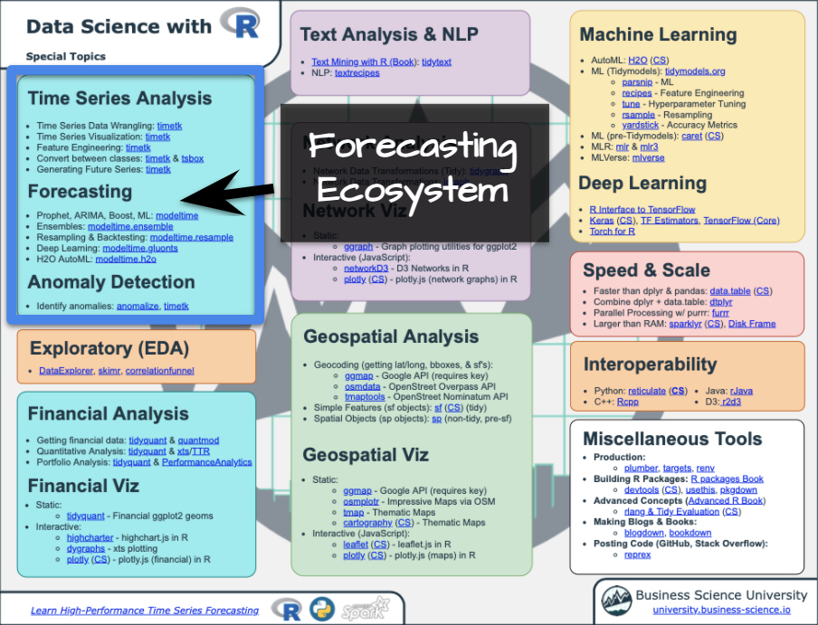
Forecasting Ecosystem Links (Ultimate R Cheat Sheet)
80/20 Recursive Terminology
Things you’ll want to be aware of as we go through this tutorial
Autoregressive Forecast
This is an Autoregressive Forecast. We are using short-term lags (Lags < Forecast Horizon). These short-term lags are the key features of the model. They are powerful predictors, but they create missing values (NA) in the future data. We use modeltime::recursive() to manage predictions, updating lags.
Panel Data
We are processing Multi-Time Series using a single model. The model processes in batches (panels) that are separated by an ID feature. This is a scalable approach to modeling many time series.
Recursive Forecasting
This process is highly scalable. The loop size is determined by the forecast horizon, and not the number of time series. So if you have 1000 time series, but your forecast horizon is only 24 months, the recursive prediction loop is only 24 iterations.
During this iterative process, a transformer function is used to create lagged values. We are responsible for defining the transformer function, but we have a lot of tools in timetk that help us create the Transformer Function:
- You’ll see
tk_augment_lags().
- There is also
tk_augment_slidify() and more.
Libraries
First, we need to load the necessary libraries:
# Tidymodeling
library(modeltime.ensemble)
library(modeltime)
library(tidymodels)

# Base Models
library(earth)
library(glmnet)
library(xgboost)

# Core Packages
library(tidyverse)
library(lubridate)
library(timetk)
Dataset
We’ll use the m4_monthly dataset, which has four monthly time series:
- This is a single data frame
- That contains 4 time series
- Each time series is identified with an “id”
- The date and value columns specify the timestamp data and the target (feature we are predicting)
We can get a visual using timetk::plot_time_series(). Refer to the Ultimate R Cheat Sheet for documentation under time series visualization.
m4_monthly %>%
    group_by(id) %>%
    plot_time_series(
        date,
        value,
        .facet_ncol = 2,
        .interactive = FALSE
    )
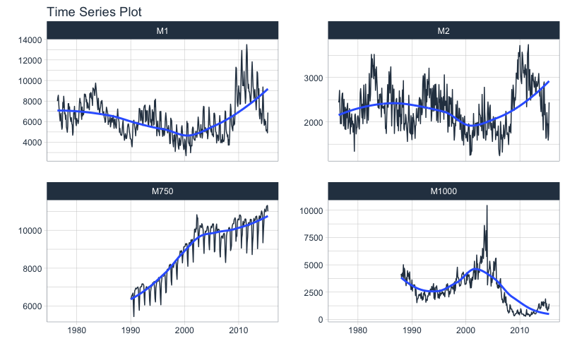
We can get a sense of the structure of the data.
- The “id” feature separates the panels.
- The “date” feature contains the timestamp information
- The “value” feature is our target for prediction (forecasting)
m4_monthly
## # A tibble: 1,574 x 3
##    id    date       value
##    <fct> <date>     <dbl>
##  1 M1    1976-06-01  8000
##  2 M1    1976-07-01  8350
##  3 M1    1976-08-01  8570
##  4 M1    1976-09-01  7700
##  5 M1    1976-10-01  7080
##  6 M1    1976-11-01  6520
##  7 M1    1976-12-01  6070
##  8 M1    1977-01-01  6650
##  9 M1    1977-02-01  6830
## 10 M1    1977-03-01  5710
## # … with 1,564 more rows
Extend with future_frame()
First, we select a forecast horizon of 24 days and extend the data frame with the function future_frame() that comes from the timetk package (Refer to the Ultimate R Cheat Sheet).
-
We do this to create a future dataset, which we can distinguish because its values will be NA.
-
The data has been extended by 24 x 4 = 96 rows.
FORECAST_HORIZON <- 24

m4_extended <- m4_monthly %>%
    group_by(id) %>%
    future_frame(
        .length_out = FORECAST_HORIZON,
        .bind_data  = TRUE
    ) %>%
    ungroup()

m4_extended
## # A tibble: 1,670 x 3
##    id    date       value
##    <fct> <date>     <dbl>
##  1 M1    1976-06-01  8000
##  2 M1    1976-07-01  8350
##  3 M1    1976-08-01  8570
##  4 M1    1976-09-01  7700
##  5 M1    1976-10-01  7080
##  6 M1    1976-11-01  6520
##  7 M1    1976-12-01  6070
##  8 M1    1977-01-01  6650
##  9 M1    1977-02-01  6830
## 10 M1    1977-03-01  5710
## # … with 1,660 more rows
Then we create a Transformer Function that will be in charge of generating the lags for each time series up to each forecasting horizon. Note that this time we use grouped lags to generate lags by group. This is important when we have multiple time series. Make sure to ungroup after the lagging process.
lag_transformer_grouped <- function(data){
    data %>%
        group_by(id) %>%
        tk_augment_lags(value, .lags = 1:FORECAST_HORIZON) %>%
        ungroup()
}
Then, we apply the function and divide the data into training and future set. Note that the tail of the data has NA values in the lagged regressors, which makes the problem a Recursive Forecasting problem.
m4_lags <- m4_extended %>%
    lag_transformer_grouped()

m4_lags %>% tail(FORECAST_HORIZON)
## # A tibble: 24 x 27
##    id    date       value value_lag1 value_lag2 value_lag3 value_lag4 value_lag5
##    <fct> <date>     <dbl>      <dbl>      <dbl>      <dbl>      <dbl>      <dbl>
##  1 M1000 2015-07-01    NA       1430        970       1140        800        880
##  2 M1000 2015-08-01    NA         NA       1430        970       1140        800
##  3 M1000 2015-09-01    NA         NA         NA       1430        970       1140
##  4 M1000 2015-10-01    NA         NA         NA         NA       1430        970
##  5 M1000 2015-11-01    NA         NA         NA         NA         NA       1430
##  6 M1000 2015-12-01    NA         NA         NA         NA         NA         NA
##  7 M1000 2016-01-01    NA         NA         NA         NA         NA         NA
##  8 M1000 2016-02-01    NA         NA         NA         NA         NA         NA
##  9 M1000 2016-03-01    NA         NA         NA         NA         NA         NA
## 10 M1000 2016-04-01    NA         NA         NA         NA         NA         NA
## # … with 14 more rows, and 19 more variables: value_lag6 <dbl>,
## #   value_lag7 <dbl>, value_lag8 <dbl>, value_lag9 <dbl>, value_lag10 <dbl>,
## #   value_lag11 <dbl>, value_lag12 <dbl>, value_lag13 <dbl>, value_lag14 <dbl>,
## #   value_lag15 <dbl>, value_lag16 <dbl>, value_lag17 <dbl>, value_lag18 <dbl>,
## #   value_lag19 <dbl>, value_lag20 <dbl>, value_lag21 <dbl>, value_lag22 <dbl>,
## #   value_lag23 <dbl>, value_lag24 <dbl>
Data Split
We split into training data and future data.
- The train data is prepared for training.
- The future data will be used later when we forecast.
train_data <- m4_lags %>%
    drop_na()

future_data <- m4_lags %>%
    filter(is.na(value))
Training the Submodels
Next, we are going to create two models that we will then join into an ensemble.
-
The first model is an Elastic Net (GLMNET) model: An elastic net applies is an improved version of linear regression that applies a penalty to the lagged regressors preventing bad lags from dominating the results. This can show an improvement versus a standard Linear Regression.
-
The second model is an XGBOOST model: An xgboost model is a tree-based algorithm that is very different in how it models vs a linear model. It’s much better for non-linear data (e.g. seasonality).
model_fit_glmnet <- linear_reg(penalty = 1) %>%
    set_engine("glmnet") %>%
    fit(value ~ ., data = train_data)

model_fit_xgboost <- boost_tree("regression", learn_rate = 0.35) %>%
    set_engine("xgboost") %>%
    fit(value ~ ., data = train_data)
Create a Recursive Ensemble
The next step is to create an ensemble with modeltime.ensemble (Refer to the Ultimate R Cheat Sheet).
We’ll use a Weighted Ensemble ensemble_weighted() with a 40/60 loading (GLMNET-to-XGBOOST).
Right after that we use the recursive() function to create the recursive model:
-
transform: The transform function gets passed to recursive, which tells the predictions how to generate the lagged features
-
train_tail: We have to use the panel_tail() function to create the train_tail by group.
-
id: This indicates how the time series panels are grouped within the incoming dataset.
recursive_ensemble_panel <- modeltime_table(
    model_fit_glmnet,
    model_fit_xgboost
) %>%
    ensemble_weighted(loadings = c(4, 6)) %>%
    recursive(
        transform  = lag_transformer_grouped,
        train_tail = panel_tail(train_data, id, FORECAST_HORIZON),
        id         = "id"
    )

recursive_ensemble_panel
## Recursive [modeltime ensemble]
##
## ── Modeltime Ensemble ───────────────────────────────────────────
## Ensemble of 2 Models (WEIGHTED)
##
## # Modeltime Table
## # A tibble: 2 x 4
##   .model_id .model   .model_desc .loadings
##       <int> <list>   <chr>           <dbl>
## 1         1 <fit[+]> GLMNET            0.4
## 2         2 <fit[+]> XGBOOST           0.6
Modeltime Table
Next, we add the recursive ensemble to the modeltime_table(), which organizes one or more models prior to forecasting. Refer to the Ultimate R Cheat Sheet for the full Modeltime Documentation with Workflow.
model_tbl <- modeltime_table(
    recursive_ensemble_panel
)

model_tbl
## # Modeltime Table
## # A tibble: 1 x 3
##   .model_id .model         .model_desc
##       <int> <list>         <chr>
## 1         1 <ensemble [2]> RECURSIVE ENSEMBLE (WEIGHTED): 2 MODELS
Forecast the Ensemble
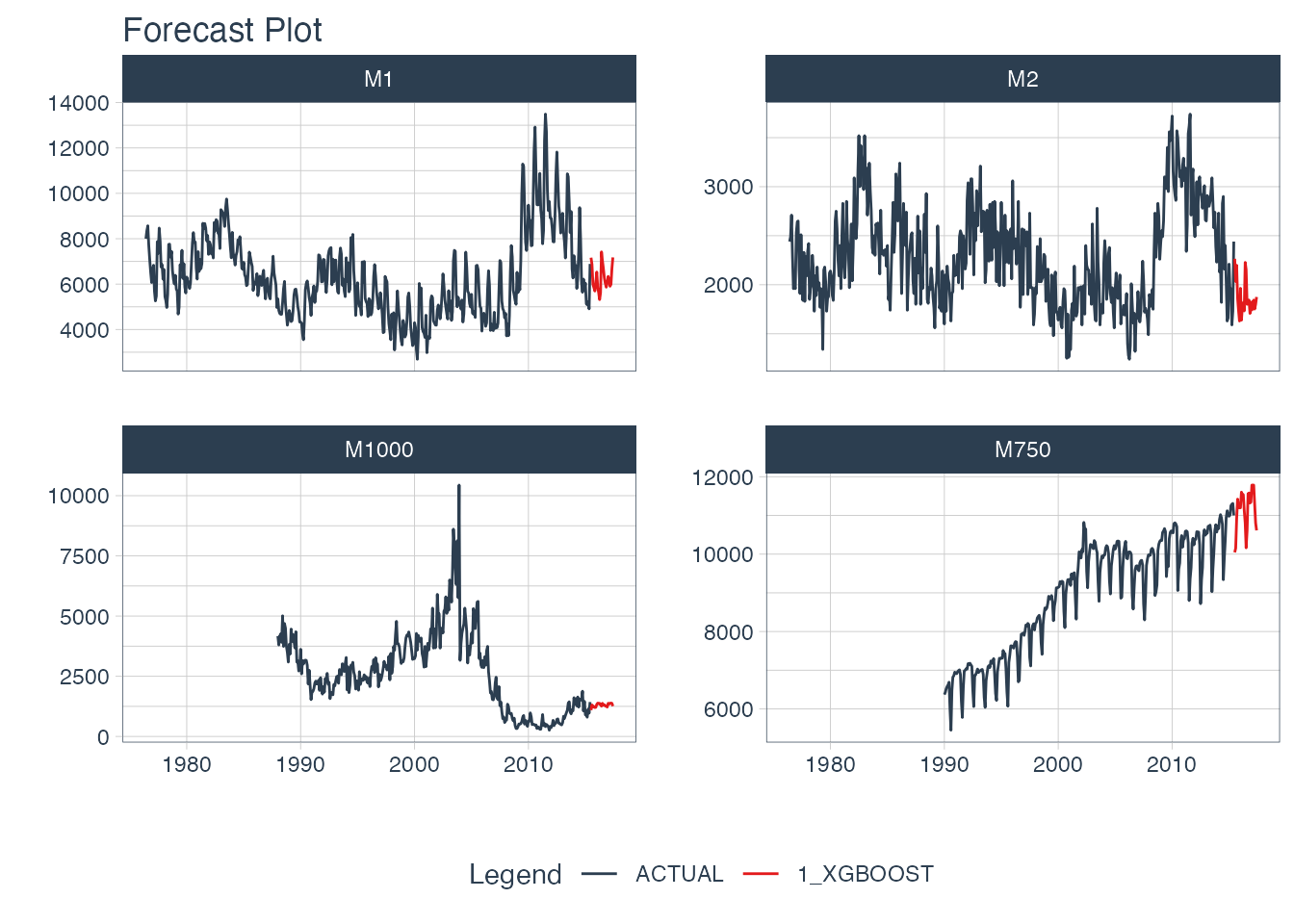
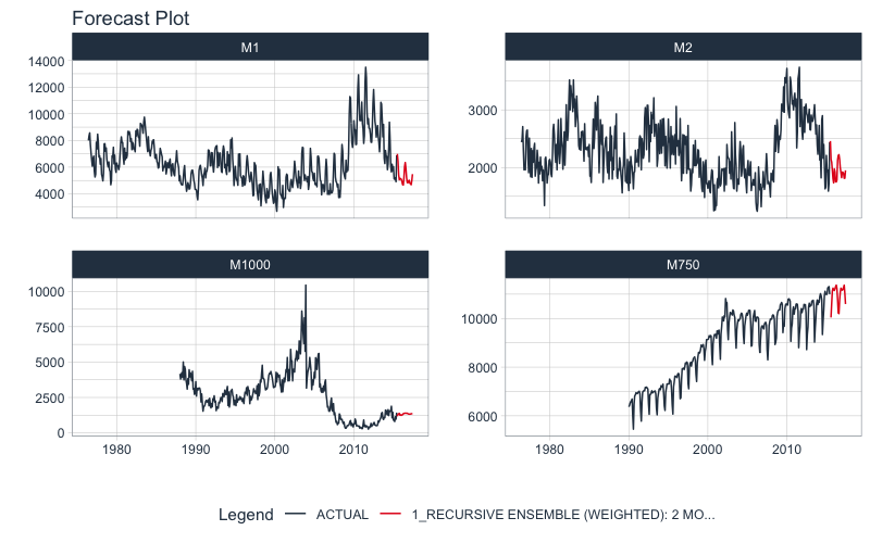
Finally, we forecast over our dataset and visualize the forecast by following the Modeltime Workflow.
- Use
modeltime_forecast() to make the forecast
- Use
plot_modeltime_forecast() to visualize the predictions
model_tbl %>%
    modeltime_forecast(
        new_data    = future_data,
        actual_data = m4_lags,
        keep_data   = TRUE
    ) %>%
    group_by(id) %>%
    plot_modeltime_forecast(
        .interactive        = FALSE,
        .conf_interval_show = FALSE,
        .facet_ncol         = 2
    )
It gets better
You’ve just scratched the surface, here’s what’s coming…
The Modeltime Ecosystem functionality is much more feature-rich than what we’ve covered here (I couldn’t possibly cover everything in this post). 😀
Here’s what I didn’t cover:
-
Feature Engineering: We can make this forecast much more accurate by including features from competition-winning strategies
-
Hyperparameter Tuning for Time Series: We can vastly improve our models by tuning them, but you need to understand how to tune for time series.
-
Deep Learning: We can use GluonTS Deep Learning for developing high-performance, scalable forecasts.
So how are you ever going to learn time series analysis and forecasting?
You’re probably thinking:
- There’s so much to learn
- My time is precious
- I’ll never learn time series
I have good news that will put those doubts behind you.
You can learn time series analysis and forecasting in hours with my state-of-the-art time series forecasting course. 👇
High-Performance Time Series Course
Become the times series expert in your organization.
My High-Performance Time Series Forecasting in R course is available now. You’ll learn timetk and modeltime plus the most powerful time series forecasting techniques available like GluonTS Deep Learning. Become the times series domain expert in your organization.
👉 High-Performance Time Series Course.
You will learn:
- Time Series Foundations - Visualization, Preprocessing, Noise Reduction, & Anomaly Detection
- Feature Engineering using lagged variables & external regressors
- Hyperparameter Tuning - For both sequential and non-sequential models
- Time Series Cross-Validation (TSCV)
- Ensembling Multiple Machine Learning & Univariate Modeling Techniques (Competition Winner)
- Deep Learning with GluonTS (Competition Winner)
- and more.
Unlock the High-Performance Time Series Course
Project Roadmap, Future Work, and Contributing to Modeltime
Modeltime is a growing ecosystem of packages that work together for forecasting and time series analysis. Here are several useful links:
Acknowledgements
I’d like to acknowledge several Business Science University students that are part of the BSU Modeltime Dev Team that have helped develop modeltime::recursive(). There efforts are truly appreciated.
- Alberto González Almuiña has helped BIG TIME with development of
modeltime::recursive() contributing the panel forecast software design.
Have questions about Modeltime Recursive?
Make a comment in the chat below. 👇
And, if you plan on using modeltime for your business, it’s a no-brainer - Join my Time Series Course.