Introducing Modeltime: Tidy Time Series Forecasting using Tidymodels
Written by Matt Dancho
I’m beyond excited to introduce modeltime, a new time series forecasting package designed to speed up model evaluation, selection, and forecasting. modeltime does this by integrating the tidymodels machine learning ecosystem of packages into a streamlined workflow for tidyverse forecasting. Follow the updated modeltime article to get started with modeltime.
- We’ll first showcase the Modeltime Ecosystem at a glance
- We’ll then explain the benefits of
modeltime
- Then we’ll go through a full Modeltime Workflow where you’ll build Automatic (Prophet, ARIMA), Machine Learning (Elastic Net, Random Forest), and Hybrid (Prophet-XGBoost) Models with Modeltime
If you like what you see, I have an Advanced Time Series Course where you will become the time-series expert for your organization by learning modeltime and timetk.
Time Series Forecasting Article Guide:
This article is part of a series of software announcements on the Modeltime Forecasting Ecosystem.
-
(Start Here) Modeltime: Tidy Time Series Forecasting using Tidymodels
-
Modeltime H2O: Forecasting with H2O AutoML
-
Modeltime Ensemble: Time Series Forecast Stacking
-
Modeltime Recursive: Tidy Autoregressive Forecasting
-
Hyperparameter Tuning Forecasts in Parallel with Modeltime
-
Time Series Forecasting Course: Now Available
Like these articles?
👉 Register to stay in the know
👈
on new cutting-edge R software like modeltime.
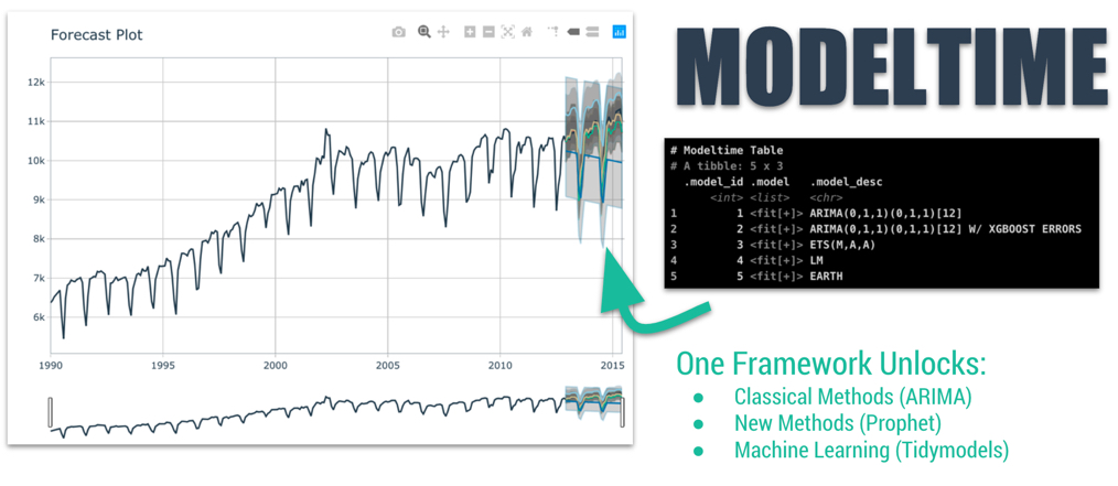
Meet the Modeltime Ecosystem
A growing ecosystem for tidymodels forecasting
Modeltime is part of a growing ecosystem of Modeltime forecasting packages. The main purpose of the Modeltime Ecosystem is to develop scalable forecasting systems.
Modeltime
The forecasting framework for the tidymodels ecosystem
modeltime is a new package designed for rapidly developing and testing time series models using machine learning models, classical models, and automated models. There are three key benefits:
-
Systematic Workflow for Forecasting. Learn a few key functions like modeltime_table(), modeltime_calibrate(), and modeltime_refit() to develop and train time series models.
-
Unlocks Tidymodels for Forecasting. Gain the benefit of all or the parsnip models including boost_tree() (XGBoost, C5.0), linear_reg() (GLMnet, Stan, Linear Regression), rand_forest() (Random Forest), and more
-
New Time Series Boosted Models including Boosted ARIMA (arima_boost()) and Boosted Prophet (prophet_boost()) that can improve accuracy by applying XGBoost model to the errors
Get the Cheat Sheet
As you go through this tutorial, it may help to use the Ultimate R Cheat Sheet. Page 3 Covers the Modeltime Forecasting Ecosystem with links to key documentation.
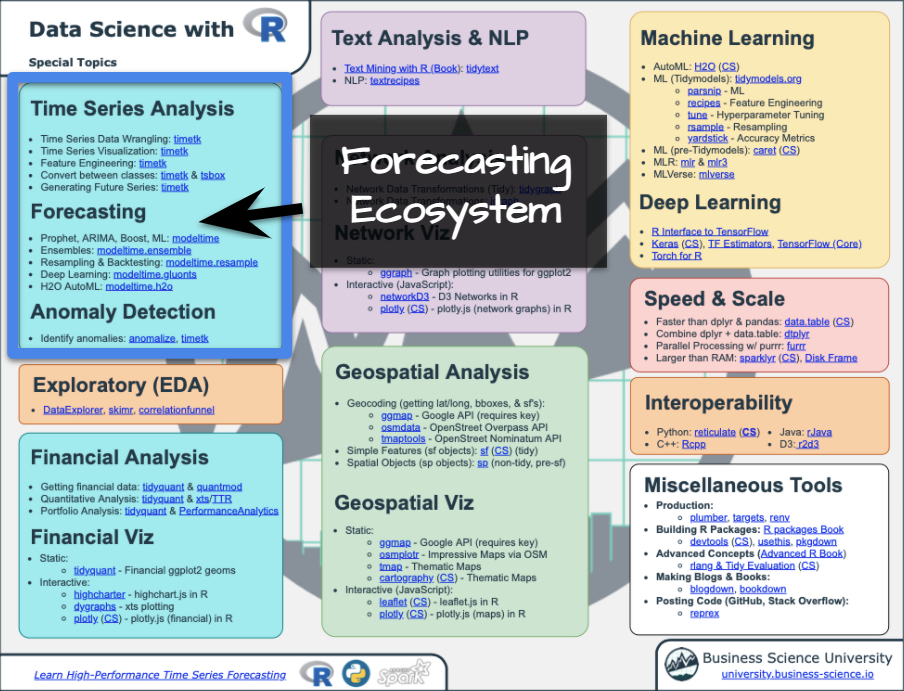
Forecasting Ecosystem Links (Ultimate R Cheat Sheet)
Getting Started
Let’s kick the tires on modeltime
Install modeltime.
install.packages("modeltime")
Load the following libraries.
library(tidymodels)
library(modeltime)
library(timetk)
library(lubridate)
library(tidyverse)
Get Your Data
Forecasting daily bike transactions
We’ll start with a bike_sharing_daily time series data set that includes bike transactions. We’ll simplify the data set to a univariate time series with columns, “date” and “value”.
bike_transactions_tbl <- bike_sharing_daily %>%
  select(dteday, cnt) %>%
  set_names(c("date", "value"))

bike_transactions_tbl
## # A tibble: 731 x 2
##    date       value
##    <date>     <dbl>
##  1 2011-01-01   985
##  2 2011-01-02   801
##  3 2011-01-03  1349
##  4 2011-01-04  1562
##  5 2011-01-05  1600
##  6 2011-01-06  1606
##  7 2011-01-07  1510
##  8 2011-01-08   959
##  9 2011-01-09   822
## 10 2011-01-10  1321
## # … with 721 more rows
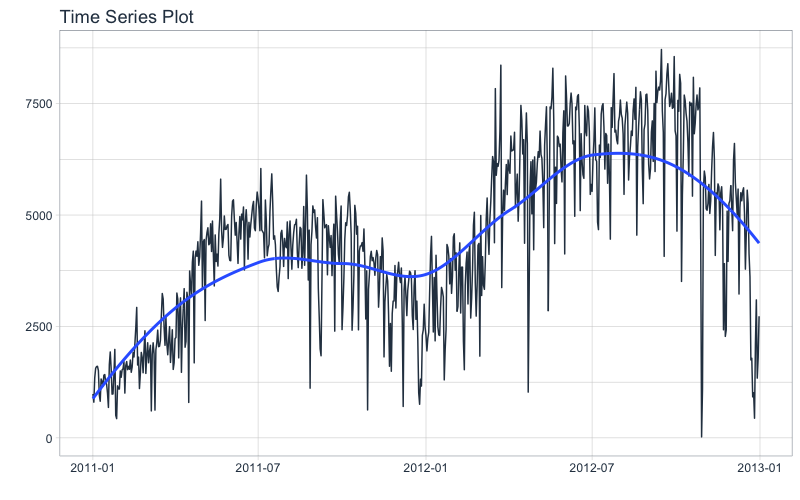
Next, visualize the dataset with the plot_time_series() function. Toggle .interactive = TRUE to get a plotly interactive plot. FALSE returns a ggplot2 static plot.
bike_transactions_tbl %>%
  plot_time_series(date, value, .interactive = FALSE)
Train / Test
Split your time series into training and testing sets
Next, use time_series_split() to make a train/test set.
- Setting
assess = "3 months" tells the function to use the last 3-months of data as the testing set.
- Setting
cumulative = TRUE tells the sampling to use all of the prior data as the training set.
splits <- bike_transactions_tbl %>%
  time_series_split(assess = "3 months", cumulative = TRUE)
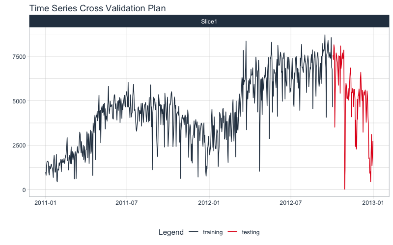
Next, visualize the train/test split.
tk_time_series_cv_plan(): Converts the splits object to a data frameplot_time_series_cv_plan(): Plots the time series sampling data using the “date” and “value” columns.
splits %>%
  tk_time_series_cv_plan() %>%
  plot_time_series_cv_plan(date, value, .interactive = FALSE)
Modeling
This is exciting.
Now for the fun part! Let’s make some models using functions from modeltime and parsnip.
1. Automatic Models
Automatic models are generally modeling approaches that have been automated. This includes “Auto ARIMA” and “Auto ETS” functions from forecast and the “Prophet” algorithm from prophet. These algorithms have been integrated into modeltime. The process is simple to set up:
- Model Spec: Use a specification function (e.g.
arima_reg(), prophet_reg()) to initialize the algorithm and key parameters
- Engine: Set an engine using one of the engines available for the Model Spec.
- Fit Model: Fit the model to the training data
Let’s make several models to see this process in action.
Auto ARIMA
Here’s the basic Auto Arima Model fitting process.
- Model Spec:
arima_reg() <– This sets up your general model algorithm and key parameters
- Set Engine:
set_engine("auto_arima") <– This selects the specific package-function to use and you can add any function-level arguments here.
- Fit Model:
fit(value ~ date, training(splits)) <– All modeltime models require a date column to be a regressor.
model_fit_arima <- arima_reg() %>%
  set_engine("auto_arima") %>%
  fit(value ~ date, training(splits))
## frequency = 7 observations per 1 week
model_fit_arima
## parsnip model object
##
## Fit time:  313ms
## Series: outcome
## ARIMA(0,1,3) with drift
##
## Coefficients:
##           ma1      ma2      ma3   drift
##       -0.6106  -0.1868  -0.0673  9.3169
## s.e.   0.0396   0.0466   0.0398  4.6225
##
## sigma^2 estimated as 730568:  log likelihood=-5227.22
## AIC=10464.44   AICc=10464.53   BIC=10486.74
Prophet
Prophet is specified just like Auto ARIMA. Note that I’ve changed to prophet_reg() and I’m supplying seasonality_yearly = TRUE).
model_fit_prophet <- prophet_reg(seasonality_yearly = TRUE) %>%
  set_engine("prophet") %>%
  fit(value ~ date, training(splits))

model_fit_prophet
## parsnip model object
##
## Fit time:  145ms
## PROPHET Model
## - growth: 'linear'
## - n.changepoints: 25
## - seasonality.mode: 'additive'
## - extra_regressors: 0
2. Machine Learning Models
Machine learning models are more complex than the automated models. This complexity typically requires a workflow (sometimes called a pipeline in other languages). The general process goes like this:
- Create Preprocessing Recipe
- Create Model Specifications
- Use Workflow to combine Model Spec and Preprocessing, and Fit Model
Preprocessing Recipe
First, I’ll create a preprocessing recipe using recipe() and adding time series steps. The process uses the “date” column to create 45 new features that I’d like to model. These include time-series signature features and fourier series.
recipe_spec <- recipe(value ~ date, training(splits)) %>%
  step_timeseries_signature(date) %>%
  step_rm(contains("am.pm"), contains("hour"), contains("minute"),
          contains("second"), contains("xts")) %>%
  step_fourier(date, period = 365, K = 5) %>%
  step_dummy(all_nominal())

recipe_spec %>% prep() %>% juice()
## # A tibble: 641 x 47
##    date       value date_index.num date_year date_year.iso date_half
##    <date>     <dbl>          <int>     <int>         <int>     <int>
##  1 2011-01-01   985     1293840000      2011          2010         1
##  2 2011-01-02   801     1293926400      2011          2010         1
##  3 2011-01-03  1349     1294012800      2011          2011         1
##  4 2011-01-04  1562     1294099200      2011          2011         1
##  5 2011-01-05  1600     1294185600      2011          2011         1
##  6 2011-01-06  1606     1294272000      2011          2011         1
##  7 2011-01-07  1510     1294358400      2011          2011         1
##  8 2011-01-08   959     1294444800      2011          2011         1
##  9 2011-01-09   822     1294531200      2011          2011         1
## 10 2011-01-10  1321     1294617600      2011          2011         1
## # … with 631 more rows, and 41 more variables: date_quarter <int>,
## #   date_month <int>, date_day <int>, date_wday <int>, date_mday <int>,
## #   date_qday <int>, date_yday <int>, date_mweek <int>, date_week <int>,
## #   date_week.iso <int>, date_week2 <int>, date_week3 <int>, date_week4 <int>,
## #   date_mday7 <int>, date_sin365_K1 <dbl>, date_cos365_K1 <dbl>,
## #   date_sin365_K2 <dbl>, date_cos365_K2 <dbl>, date_sin365_K3 <dbl>,
## #   date_cos365_K3 <dbl>, date_sin365_K4 <dbl>, date_cos365_K4 <dbl>,
## #   date_sin365_K5 <dbl>, date_cos365_K5 <dbl>, date_month.lbl_01 <dbl>,
## #   date_month.lbl_02 <dbl>, date_month.lbl_03 <dbl>, date_month.lbl_04 <dbl>,
## #   date_month.lbl_05 <dbl>, date_month.lbl_06 <dbl>, date_month.lbl_07 <dbl>,
## #   date_month.lbl_08 <dbl>, date_month.lbl_09 <dbl>, date_month.lbl_10 <dbl>,
## #   date_month.lbl_11 <dbl>, date_wday.lbl_1 <dbl>, date_wday.lbl_2 <dbl>,
## #   date_wday.lbl_3 <dbl>, date_wday.lbl_4 <dbl>, date_wday.lbl_5 <dbl>,
## #   date_wday.lbl_6 <dbl>
With a recipe in-hand, we can set up our machine learning pipelines.
Elastic Net
Making an Elastic NET model is easy to do. Just set up your model spec using linear_reg() and set_engine("glmnet"). Note that we have not fitted the model yet (as we did in previous steps).
model_spec_glmnet <- linear_reg(penalty = 0.01, mixture = 0.5) %>%
  set_engine("glmnet")
Next, make a fitted workflow:
- Start with a
workflow()
- Add a Model Spec:
add_model(model_spec_glmnet)
- Add Preprocessing:
add_recipe(recipe_spec %>% step_rm(date)) <– Note that I’m removing the “date” column since Machine Learning algorithms don’t typically know how to deal with date or date-time features
- Fit the Workflow:
fit(training(splits))
workflow_fit_glmnet <- workflow() %>%
  add_model(model_spec_glmnet) %>%
  add_recipe(recipe_spec %>% step_rm(date)) %>%
  fit(training(splits))
Random Forest
We can fit a Random Forest using a similar process as the Elastic Net.
model_spec_rf <- rand_forest(trees = 500, min_n = 50) %>%
  set_engine("randomForest")

workflow_fit_rf <- workflow() %>%
  add_model(model_spec_rf) %>%
  add_recipe(recipe_spec %>% step_rm(date)) %>%
  fit(training(splits))
3. Hybrid ML Models
I’ve included several hybrid models (e.g. arima_boost() and prophet_boost()) that combine both automated algorithms with machine learning. I’ll showcase prophet_boost() next!
Prophet Boost
The Prophet Boost algorithm combines Prophet with XGBoost to get the best of both worlds (i.e. Prophet Automation + Machine Learning). The algorithm works by:
- First modeling the univariate series using Prophet
- Using regressors supplied via the preprocessing recipe (remember our recipe generated 45 new features), and regressing the Prophet Residuals with the XGBoost model
We can set the model up using a workflow just like with the machine learning algorithms.
model_spec_prophet_boost <- prophet_boost(seasonality_yearly = TRUE) %>%
  set_engine("prophet_xgboost")

workflow_fit_prophet_boost <- workflow() %>%
  add_model(model_spec_prophet_boost) %>%
  add_recipe(recipe_spec) %>%
  fit(training(splits))

workflow_fit_prophet_boost
## ══ Workflow [trained] ═════════════════════════════════════════════════════════════════════════════════
## Preprocessor: Recipe
## Model: prophet_boost()
##
## ── Preprocessor ───────────────────────────────────────────────────────────────────────────────────────
## 4 Recipe Steps
##
## ● step_timeseries_signature()
## ● step_rm()
## ● step_fourier()
## ● step_dummy()
##
## ── Model ──────────────────────────────────────────────────────────────────────────────────────────────
## PROPHET w/ XGBoost Errors
## ---
## Model 1: PROPHET
## - growth: 'linear'
## - n.changepoints: 25
## - seasonality.mode: 'additive'
##
## ---
## Model 2: XGBoost Errors
##
## xgboost::xgb.train(params = list(eta = 0.3, max_depth = 6, gamma = 0,
##     colsample_bytree = 1, min_child_weight = 1, subsample = 1),
##     data = x, nrounds = 15, watchlist = wlist, verbose = 0, objective = "reg:squarederror",
##     nthread = 1)
The Modeltime Workflow
Speed up model evaluation and selection with modeltime
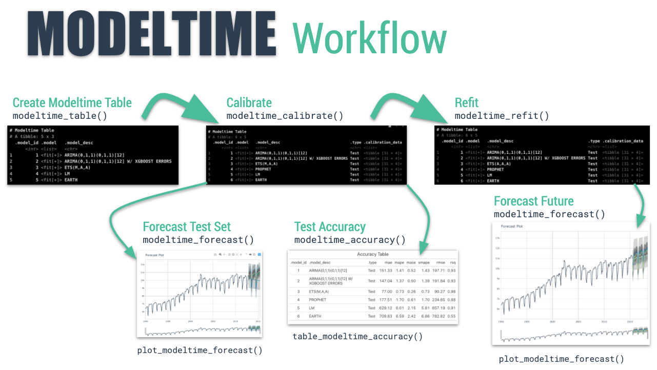
The modeltime workflow is designed to speed up model evaluation and selection. Now that we have several time series models, let’s analyze them and forecast the future with the modeltime workflow.
Modeltime Table
The Modeltime Table organizes the models with IDs and creates generic descriptions to help us keep track of our models. Let’s add the models to a modeltime_table().
model_table <- modeltime_table(
  model_fit_arima,
  model_fit_prophet,
  workflow_fit_glmnet,
  workflow_fit_rf,
  workflow_fit_prophet_boost
)

model_table
## # Modeltime Table
## # A tibble: 5 x 3
##   .model_id .model     .model_desc
##       <int> <list>     <chr>
## 1         1 <fit[+]>   ARIMA(0,1,3) WITH DRIFT
## 2         2 <fit[+]>   PROPHET
## 3         3 <workflow> GLMNET
## 4         4 <workflow> RANDOMFOREST
## 5         5 <workflow> PROPHET W/ XGBOOST ERRORS
Calibration
Model Calibration is used to quantify error and estimate confidence intervals. We’ll perform model calibration on the out-of-sample data (aka. the Testing Set) with the modeltime_calibrate() function. Two new columns are generated (“.type” and “.calibration_data”), the most important of which is the “.calibration_data”. This includes the actual values, fitted values, and residuals for the testing set.
calibration_table <- model_table %>%
  modeltime_calibrate(testing(splits))

calibration_table
## # Modeltime Table
## # A tibble: 5 x 5
##   .model_id .model     .model_desc               .type .calibration_data
##       <int> <list>     <chr>                     <chr> <list>
## 1         1 <fit[+]>   ARIMA(0,1,3) WITH DRIFT   Test  <tibble [90 × 4]>
## 2         2 <fit[+]>   PROPHET                   Test  <tibble [90 × 4]>
## 3         3 <workflow> GLMNET                    Test  <tibble [90 × 4]>
## 4         4 <workflow> RANDOMFOREST              Test  <tibble [90 × 4]>
## 5         5 <workflow> PROPHET W/ XGBOOST ERRORS Test  <tibble [90 × 4]>
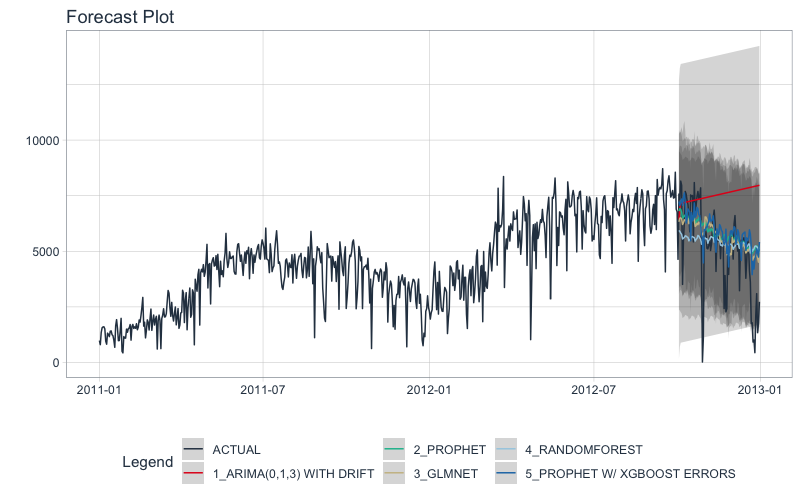
Forecast (Testing Set)
With calibrated data, we can visualize the testing predictions (forecast).
- Use
modeltime_forecast() to generate the forecast data for the testing set as a tibble.
- Use
plot_modeltime_forecast() to visualize the results in interactive and static plot formats.
calibration_table %>%
  modeltime_forecast(actual_data = bike_transactions_tbl) %>%
  plot_modeltime_forecast(.interactive = FALSE)
Accuracy (Testing Set)
Next, calculate the testing accuracy to compare the models.
- Use
modeltime_accuracy() to generate the out-of-sample accuracy metrics as a tibble.
- Use
table_modeltime_accuracy() to generate interactive and static
calibration_table %>%
  modeltime_accuracy() %>%
  table_modeltime_accuracy(.interactive = FALSE)
| .model_id |
.model_desc |
.type |
mae |
mape |
mase |
smape |
rmse |
rsq |
| 1 |
ARIMA(0,1,3) WITH DRIFT |
Test |
2540.11 |
474.89 |
2.74 |
46.00 |
3188.09 |
0.39 |
| 2 |
PROPHET |
Test |
1221.18 |
365.13 |
1.32 |
28.68 |
1764.93 |
0.44 |
| 3 |
GLMNET |
Test |
1197.06 |
340.57 |
1.29 |
28.44 |
1650.87 |
0.49 |
| 4 |
RANDOMFOREST |
Test |
1309.79 |
327.88 |
1.42 |
30.24 |
1809.05 |
0.47 |
| 5 |
PROPHET W/ XGBOOST ERRORS |
Test |
1189.28 |
332.44 |
1.28 |
28.48 |
1644.25 |
0.55 |
Analyze Results
From the accuracy measures and forecast results, we see that:
- Auto ARIMA model is not a good fit for this data.
- The best model is Prophet + XGBoost
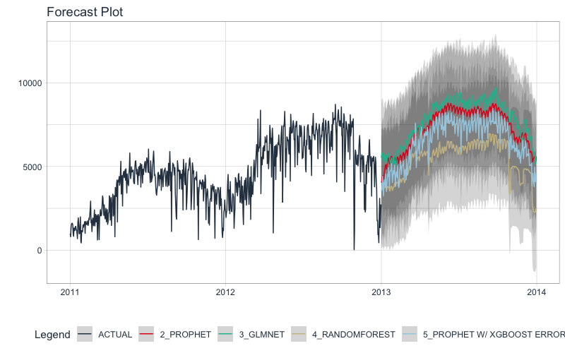
Let’s exclude the Auto ARIMA from our final model, then make future forecasts with the remaining models.
Refit and Forecast Forward
Refitting is a best-practice before forecasting the future.
modeltime_refit(): We re-train on full data (bike_transactions_tbl)modeltime_forecast(): For models that only depend on the “date” feature, we can use h (horizon) to forecast forward. Setting h = "12 months" forecasts then next 12-months of data.
calibration_table %>%
  # Remove ARIMA model with low accuracy
  filter(.model_id != 1) %>%

  # Refit and Forecast Forward
  modeltime_refit(bike_transactions_tbl) %>%
  modeltime_forecast(h = "12 months", actual_data = bike_transactions_tbl) %>%
  plot_modeltime_forecast(.interactive = FALSE)
It gets better
You’ve just scratched the surface, here’s what’s coming…
The modeltime package functionality is much more feature-rich than what we’ve covered here (I couldn’t possibly cover everything in this post). 😀
Here’s what I didn’t cover:
-
Feature Engineering: The art of time series analysis is feature engineering. Modeltime works with cutting-edge time-series preprocessing tools including those in recipes and timetk packages.
-
Hyper Parameter Tuning: ARIMA models and Machine Learning models can be tuned. There’s a right and a wrong way (and it’s not the same for both types).
-
Scalability: Training multiple time series groups and automation is a huge need area in organizations. You need to know how to scale your analyses to thousands of time series.
-
Strengths and Weaknesses: Did you know certain machine learning models are better for trend, seasonality, but not both? Why is ARIMA way better for certain datasets? When will Random Forest and XGBoost fail?
-
Deep Learning: Recurrent Neural Networks (RRNs) have been crushing time series competitions. Will they work for business data? How can you implement them?
So how are you ever going to learn time series analysis and forecasting?
You’re probably thinking:
- There’s so much to learn
- My time is precious
- I’ll never learn time series
I have good news that will put those doubts behind you.
You can learn time series analysis and forecasting in hours with my state-of-the-art time series forecasting course. 👇
High-Performance Time Series Course
Become the times series expert in your organization.
My High-Performance Time Series Forecasting in R course is available now. You’ll learn timetk and modeltime plus the most powerful time series forecasting techniques available like GluonTS Deep Learning. Become the times series domain expert in your organization.
👉 High-Performance Time Series Course.
You will learn:
- Time Series Foundations - Visualization, Preprocessing, Noise Reduction, & Anomaly Detection
- Feature Engineering using lagged variables & external regressors
- Hyperparameter Tuning - For both sequential and non-sequential models
- Time Series Cross-Validation (TSCV)
- Ensembling Multiple Machine Learning & Univariate Modeling Techniques (Competition Winner)
- Deep Learning with GluonTS (Competition Winner)
- and more.
Unlock the High-Performance Time Series Course
Project Roadmap, Future Work, and Contributing to Modeltime
Modeltime is a growing ecosystem of packages that work together for forecasting and time series analysis. Here are several useful links:
Have questions about modeltime?
Make a comment in the chat below. 👇
And, if you plan on using modeltime for your business, it’s a no-brainer - Join my Time Series Course (it’s really insane).