Introducing Modeltime H2O: Automatic Forecasting with H2O AutoML
Written by Matt Dancho and Alberto González Almuiña
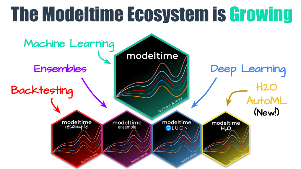
I’m beyond excited to introduce modeltime.h2o, the time series forecasting package that integrates H2O AutoML (Automatic Machine Learning) as a Modeltime Forecasting Backend. This tutorial (view the original article here) introduces our new R Package, Modeltime H2O.
- We’ll quickly introduce you to the growing modeltime ecosystem.
- Then, we’ll forecast with H2O AutoML using the
modeltime.h2o backend
If you like what you see, I have an Advanced Time Series Course where you will learn the foundations of the growing Modeltime Ecosystem.
Time Series Forecasting Article Guide:
This article is part of a series of software announcements on the Modeltime Forecasting Ecosystem.
-
(Start Here) Modeltime: Tidy Time Series Forecasting using Tidymodels
-
Modeltime H2O: Forecasting with H2O AutoML
-
Modeltime Ensemble: Time Series Forecast Stacking
-
Modeltime Recursive: Tidy Autoregressive Forecasting
-
Hyperparameter Tuning Forecasts in Parallel with Modeltime
-
Time Series Forecasting Course: Now Available
Like these articles?
👉 Register to stay in the know
👈
on new cutting-edge R software like modeltime.
Meet the Modeltime Ecosystem
A growing ecosystem for tidymodels forecasting
Modeltime H2O is part of a growing ecosystem of Modeltime forecasting packages. The main purpose of the Modeltime Ecosystem is to develop scalable forecasting systems.
Modeltime H2O
The H2O AutoML backend for Modeltime

Modeltime H2O provides an H2O backend to the Modeltime Forecasting Ecosystem. The main algorithm is H2O AutoML, an automatic machine learning library that is built for speed and scale.
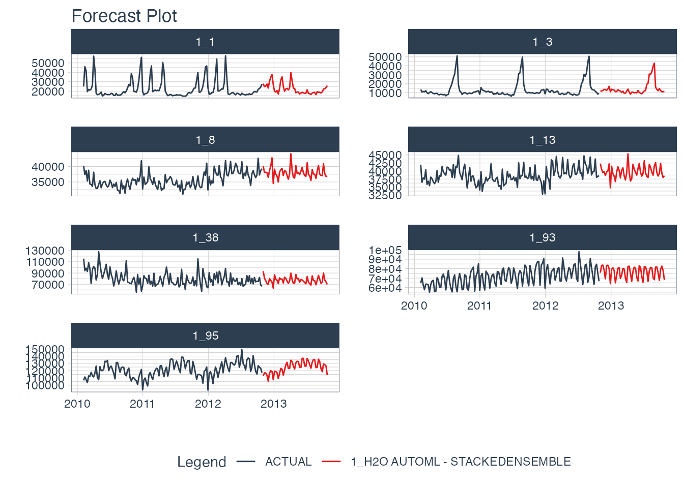
This forecast was created with H2O AutoML. We’ll make this forecast in our short tutorial.
Getting Started with Modeltime H2O
Forecasting with modeltime.h2o made easy! This short tutorial shows how you can use:
-
H2O AutoML for forecasting implemented via automl_reg(). This function trains and cross-validates multiple machine learning and deep learning models (XGBoost GBM, GLMs, Random Forest, GBMs…) and then trains two Stacked Ensembled models, one of all the models, and one of only the best models of each kind. Finally, the best model is selected based on a stopping metric. And we take care of all this for you!
-
Save & Load Models functionality to ensure the persistence of your models.
Get the Cheat Sheet
As you go through this tutorial, it may help to use the Ultimate R Cheat Sheet. Page 3 Covers the Modeltime Forecasting Ecosystem with links to key documentation.
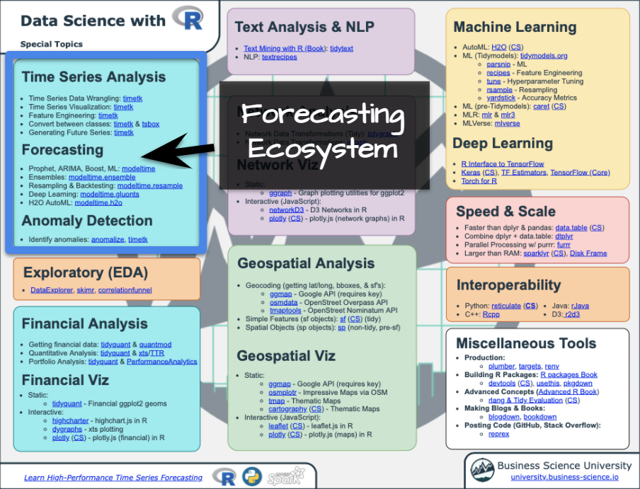
Forecasting Ecosystem Links (Ultimate R Cheat Sheet)
Libraries
The modeltime.h2o package is now on CRAN:
# Install Modeltime H2O from CRAN
install.packages("modeltime.h2o")
Load the following libraries:
library(tidymodels)
library(modeltime.h2o)
library(tidyverse)
library(timetk)
Collect data and split into training and test sets
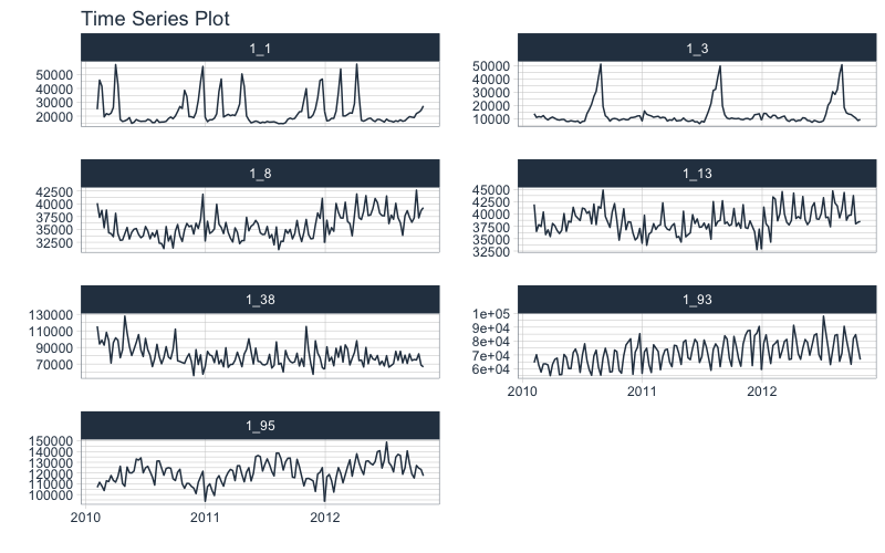
Next, we load the walmart_sales_weekly data containing 7 time series and visualize them using the timetk::plot_time_series() function.
data_tbl <- walmart_sales_weekly %>%
    select(id, Date, Weekly_Sales)

data_tbl %>%
  group_by(id) %>%
  plot_time_series(
      .date_var    = Date,
      .value       = Weekly_Sales,
      .facet_ncol  = 2,
      .smooth      = F,
      .interactive = F
  )
Then, we separate the data with the initial_time_split() function and generate a training dataset and a test one.
splits <- time_series_split(data_tbl, assess = "3 month", cumulative = TRUE)

recipe_spec <- recipe(Weekly_Sales ~ ., data = training(splits)) %>%
    step_timeseries_signature(Date)

train_tbl <- training(splits) %>% bake(prep(recipe_spec), .)
test_tbl  <- testing(splits) %>% bake(prep(recipe_spec), .)
Model specification, training and prediction
In order to correctly use modeltime.h2o, it is necessary to connect to an H2O cluster through the h2o.init() function. You can find more information on how to set up the cluster by typing ?h2o.init or by visiting the official site.
h2o.init(
    nthreads = -1,
    ip       = 'localhost',
    port     = 54321
)

# Optional - Turn off progress indicators during training runs
h2o.no_progress()
##  Connection successful!
##
## R is connected to the H2O cluster:
##     H2O cluster uptime:         2 days 8 hours
##     H2O cluster timezone:       America/New_York
##     H2O data parsing timezone:  UTC
##     H2O cluster version:        3.32.0.1
##     H2O cluster version age:    5 months and 6 days !!!
##     H2O cluster name:           H2O_started_from_R_mdancho_rfu672
##     H2O cluster total nodes:    1
##     H2O cluster total memory:   7.70 GB
##     H2O cluster total cores:    12
##     H2O cluster allowed cores:  12
##     H2O cluster healthy:        TRUE
##     H2O Connection ip:          localhost
##     H2O Connection port:        54321
##     H2O Connection proxy:       NA
##     H2O Internal Security:      FALSE
##     H2O API Extensions:         Amazon S3, XGBoost, Algos, AutoML, Core V3, TargetEncoder, Core V4
##     R Version:                  R version 4.0.2 (2020-06-22)
Now comes the fun part! We define our model specification with the automl_reg() function and pass the arguments through the engine:
model_spec <- automl_reg(mode = 'regression') %>%
    set_engine(
         engine                     = 'h2o',
         max_runtime_secs           = 5,
         max_runtime_secs_per_model = 3,
         max_models                 = 3,
         nfolds                     = 5,
         exclude_algos              = c("DeepLearning"),
         verbosity                  = NULL,
         seed                       = 786
    )

model_spec
## H2O AutoML Model Specification (regression)
##
## Engine-Specific Arguments:
##   max_runtime_secs = 5
##   max_runtime_secs_per_model = 3
##   max_models = 3
##   nfolds = 5
##   exclude_algos = c("DeepLearning")
##   verbosity = NULL
##   seed = 786
##
## Computational engine: h2o
Next, let’s train the model!
model_fitted <- model_spec %>%
    fit(Weekly_Sales ~ ., data = train_tbl)
##                                           model_id mean_residual_deviance
## 1 StackedEnsemble_AllModels_AutoML_20210314_202927               35931457
## 2                 XGBoost_3_AutoML_20210314_202927               37716780
## 3                 XGBoost_2_AutoML_20210314_202927               39595467
## 4                 XGBoost_1_AutoML_20210314_202927               40327699
##       rmse      mse      mae     rmsle
## 1 5994.285 35931457 3624.093 0.1408371
## 2 6141.399 37716780 3778.491 0.1468337
## 3 6292.493 39595467 3932.025 0.1553225
## 4 6350.409 40327699 4089.680 0.1659641
##
## [4 rows x 6 columns]
We can check out the trained H2O AutoML model.
model_fitted
## parsnip model object
##
## Fit time:  8.1s
##
## H2O AutoML - Stackedensemble
## --------
## Model: Model Details:
## ==============
##
## H2ORegressionModel: stackedensemble
## Model ID:  StackedEnsemble_AllModels_AutoML_20210314_202927
## Number of Base Models: 3
##
## Base Models (count by algorithm type):
##
## xgboost
##       3
##
## Metalearner:
##
## Metalearner algorithm: glm
## Metalearner cross-validation fold assignment:
##   Fold assignment scheme: AUTO
##   Number of folds: 5
##   Fold column: NULL
## Metalearner hyperparameters:
##
##
## H2ORegressionMetrics: stackedensemble
## ** Reported on training data. **
##
## MSE:  14187153
## RMSE:  3766.584
## MAE:  2342.327
## RMSLE:  0.08087684
## Mean Residual Deviance :  14187153
##
##
##
## H2ORegressionMetrics: stackedensemble
## ** Reported on cross-validation data. **
## ** 5-fold cross-validation on training data (Metrics computed for combined holdout predictions) **
##
## MSE:  35931457
## RMSE:  5994.285
## MAE:  3624.093
## RMSLE:  0.1408371
## Mean Residual Deviance :  35931457
Finally, we predict on the test dataset:
predict(model_fitted, test_tbl)
## # A tibble: 84 x 1
##      .pred
##      <dbl>
##  1  18233.
##  2  31529.
##  3  37662.
##  4  40605.
##  5  74633.
##  6  81293.
##  7 134751.
##  8  17794.
##  9  36732.
## 10  37074.
## # … with 74 more rows
Modeltime Workflow
Once we have our fitted model, we can follow the Modeltime Workflow:
-
Add fitted models to a Model Table.
-
Calibrate the models to a testing set.
-
Perform Testing Set Forecast Assessment & Accuracy Evaluation.
-
Refit the models to Full Dataset & Forecast Forward
Add fitted models to a Model Table
First, we create the model table:
modeltime_tbl <- modeltime_table(
    model_fitted
)

modeltime_tbl
## # Modeltime Table
## # A tibble: 1 x 3
##   .model_id .model   .model_desc
##       <int> <list>   <chr>
## 1         1 <fit[+]> H2O AUTOML - STACKEDENSEMBLE
Calibrate & Testing Set Forecast & Accuracy Evaluation
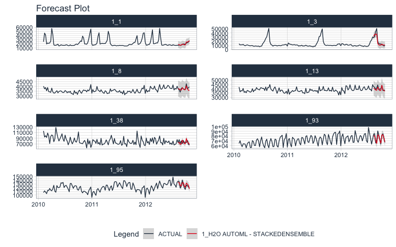
Next, we calibrate to the testing set and visualize the forecasts:
modeltime_tbl %>%
  modeltime_calibrate(test_tbl) %>%
    modeltime_forecast(
        new_data    = test_tbl,
        actual_data = data_tbl,
        keep_data   = TRUE
    ) %>%
    group_by(id) %>%
    plot_modeltime_forecast(
        .facet_ncol = 2,
        .interactive = FALSE
    )
Refit to Full Dataset & Forecast Forward
Before using refit on our dataset, let’s prepare our data. We create data_prepared_tbl which represents the complete dataset (the union of train and test) with the variables created with the recipe named recipe_spec. Subsequently, we create the dataset future_prepared_tbl that represents the dataset with the future data to one year and the required variables.
data_prepared_tbl <- bind_rows(train_tbl, test_tbl)

future_tbl <- data_prepared_tbl %>%
    group_by(id) %>%
    future_frame(.length_out = "1 year") %>%
    ungroup()

future_prepared_tbl <- bake(prep(recipe_spec), future_tbl)
Finally, we use modeltime_refit() to re-train our model on the entire dataset. This is a best-practice for improving forecast results.
refit_tbl <- modeltime_tbl %>%
    modeltime_refit(data_prepared_tbl)
##                                           model_id mean_residual_deviance
## 1 StackedEnsemble_AllModels_AutoML_20210314_202938               34093669
## 2                 XGBoost_3_AutoML_20210314_202938               37000407
## 3                 XGBoost_2_AutoML_20210314_202938               37884414
## 4                 XGBoost_1_AutoML_20210314_202938               39079782
##       rmse      mse      mae     rmsle
## 1 5838.978 34093669 3565.292 0.1407856
## 2 6082.796 37000407 3695.199 0.1446849
## 3 6155.032 37884414 3928.093 0.1623624
## 4 6251.382 39079782 4207.449 0.1819081
##
## [4 rows x 6 columns]
Let’s visualize the final forecast
We can quickly visualize the final forecast with modeltime_forecast() and it’s plotting utility function, plot_modeltime_forecast().
refit_tbl %>%
    modeltime_forecast(
        new_data    = future_prepared_tbl,
        actual_data = data_prepared_tbl,
        keep_data   = TRUE
    ) %>%
    group_by(id) %>%
    plot_modeltime_forecast(
        .facet_ncol  = 2,
        .interactive = FALSE
    )
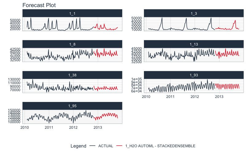
We can likely do better than this if we train longer but really good for a quick example!
Saving and Loading Models
H2O models will need to “serialized” (a fancy word for saved to a directory that contains the recipe for recreating the models). To save the models, use save_h2o_model().
- Provide a directory where you want to save the model.
- This saves the model file in the directory.
model_fitted %>%
  save_h2o_model(path = "../model_fitted", overwrite = TRUE)
You can reload the model into R using load_h2o_model().
model_h2o <- load_h2o_model(path = "../model_fitted/")
It gets better
You’ve just scratched the surface, here’s what’s coming…
The Modeltime Ecosystem functionality is much more feature-rich than what we’ve covered here (I couldn’t possibly cover everything in this post). 😀
Here’s what I didn’t cover:
-
Feature Engineering: We can make this forecast much more accurate by including features from competition-winning strategies
-
Ensemble Modeling: We can stack H2O Models with other models not included in H2O like GluonTS Deep Learning.
-
Deep Learning: We can use GluonTS Deep Learning for developing high-performance, scalable forecasts.
So how are you ever going to learn time series analysis and forecasting?
You’re probably thinking:
- There’s so much to learn
- My time is precious
- I’ll never learn time series
I have good news that will put those doubts behind you.
You can learn time series analysis and forecasting in hours with my state-of-the-art time series forecasting course. 👇
High-Performance Time Series Course
Become the times series expert in your organization.
My High-Performance Time Series Forecasting in R course is available now. You’ll learn timetk and modeltime plus the most powerful time series forecasting techniques available like GluonTS Deep Learning. Become the times series domain expert in your organization.
👉 High-Performance Time Series Course.
You will learn:
- Time Series Foundations - Visualization, Preprocessing, Noise Reduction, & Anomaly Detection
- Feature Engineering using lagged variables & external regressors
- Hyperparameter Tuning - For both sequential and non-sequential models
- Time Series Cross-Validation (TSCV)
- Ensembling Multiple Machine Learning & Univariate Modeling Techniques (Competition Winner)
- Deep Learning with GluonTS (Competition Winner)
- and more.
Unlock the High-Performance Time Series Course
Project Roadmap, Future Work, and Contributing to Modeltime
Modeltime is a growing ecosystem of packages that work together for forecasting and time series analysis. Here are several useful links:
Acknowledgements
I’d like to acknowledge several Business Science University students that are part of the BSU Modeltime Dev Team that have helped develop modeltime.h2o. There efforts are truly appreciated.
Have questions about Modeltime H2O?
Make a comment in the chat below. 👇
And, if you plan on using modeltime.h2o for your business, it’s a no-brainer - Join my Time Series Course.