Time Series in 5-Minutes, Part 5: Anomaly Detection
Written by Matt Dancho
Have 5-minutes? Then let’s learn time series. In this short articles series, I highlight how you can get up to speed quickly on important aspects of time series analysis. Today we are focusing analyzing anomalies in time series data.
Updates
This article has been updated. View the updated Time Series in 5-Minutes article at Business Science.
Time Series in 5-Mintues
Articles in this Series
Anomaly Detection - A fundamental tool in your arsenal
I just released timetk 2.0.0 (read the release announcement). A ton of new functionality has been added. We’ll discuss some of the key pieces in this article series:
👉 Register for our blog to get new articles as we release them.
Have 5-Minutes?
Then let’s learn Time Series Anomaly Detection
Anomaly detection is an important part of time series analysis:
- Detecting anomalies can signify special events
- Cleaning anomalies can improve forecast error
In this short tutorial, we will cover the plot_anomaly_diagnostics() and tk_anomaly_diagnostics() functions for visualizing and automatically detecting anomalies at scale.
Let’s Get Started
First setup the libraries we’ll use:
library(tidyverse)
library(timetk)
Data
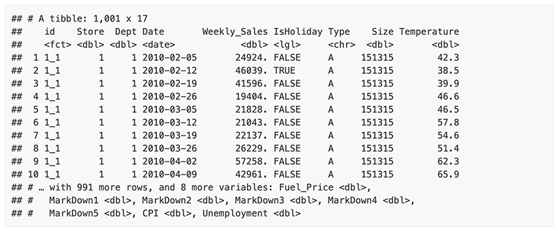
This tutorial will use the walmart_sales_weekly dataset:
- Weekly
- Sales spikes at various events
walmart_sales_weekly
Automatic Anomaly Detection
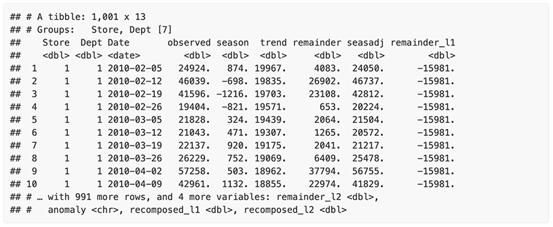
To get the data on the anomalies, we use tk_anomaly_diagnostics(), the preprocessing function.
The tk_anomaly_diagnostics() method for anomaly detection implements a 2-step process to detect outliers in time series.
Step 1: Detrend & Remove Seasonality using STL Decomposition
The decomposition separates the “season” and “trend” components from the “observed” values leaving the “remainder” for anomaly detection.
The user can control two parameters: frequency and trend.
.frequency: Adjusts the “season” component that is removed from the “observed” values..trend: Adjusts the trend window (t.window parameter from stats::stl() that is used.
The user may supply both .frequency and .trend as time-based durations (e.g. “6 weeks”) or numeric values (e.g. 180) or “auto”, which predetermines the frequency and/or trend based on the scale of the time series using the tk_time_scale_template().
Step 2: Anomaly Detection
Once “trend” and “season” (seasonality) is removed, anomaly detection is performed on the “remainder”. Anomalies are identified, and boundaries (recomposed_l1 and recomposed_l2) are determined.
The Anomaly Detection Method uses an inner quartile range (IQR) of +/-25 the median.
IQR Adjustment, alpha parameter
With the default alpha = 0.05, the limits are established by expanding the 25/75 baseline by an IQR Factor of 3 (3X). The IQR Factor = 0.15 / alpha (hence 3X with alpha = 0.05):
- To increase the IQR Factor controlling the limits, decrease the alpha, which makes it more difficult to be an outlier.
- Increase alpha to make it easier to be an outlier.
- The IQR outlier detection method is used in
forecast::tsoutliers().
- A similar outlier detection method is used by Twitter’s AnomalyDetection package.
- Both Twitter and Forecast tsoutliers methods have been implemented in Business Science’s anomalize package.
walmart_sales_weekly %>%
  group_by(Store, Dept) %>%
  tk_anomaly_diagnostics(Date, Weekly_Sales)
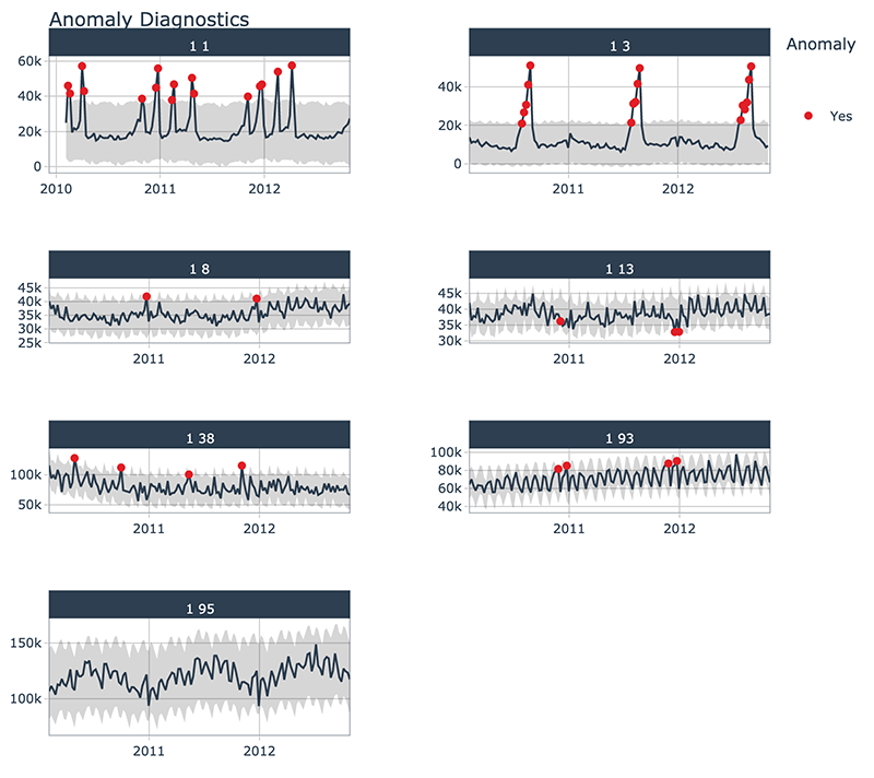
Anomaly Visualization
Using the plot_anomaly_diagnostics() function, we can interactively detect anomalies at scale.
The plot_anomaly_diagnostics() is a visualtion wrapper for tk_anomaly_diagnostics() group-wise anomaly detection, implementing the 2-step process from above.
walmart_sales_weekly %>%
  group_by(Store, Dept) %>%
  plot_anomaly_diagnostics(Date, Weekly_Sales, .facet_ncol = 2)
Have questions on using Timetk for time series?
Make a comment in the chat below. 👇
And, if you plan on using timetk for your business, it’s a no-brainer - Join the Time Series Course.