Time Series in 5-Minutes, Part 4: Seasonality
Written by Matt Dancho
Have 5-minutes? Then let’s learn time series. In this short articles series, I highlight how you can get up to speed quickly on important aspects of time series analysis. Today we are focusing on seasonality in time series data.
Updates
This article has been updated. View the updated Time Series in 5-Minutes article at Business Science.
Time Series in 5-Mintues
Articles in this Series
Seasonality - A fundamental tool in your arsenal
I just released timetk 2.0.0 (read the release announcement). A ton of new functionality has been added. We’ll discuss some of the key pieces in this article series:
👉 Register for our blog to get new articles as we release them.
Have 5-Minutes?
Then let’s learn Time Series Seasonality
A collection of tools for working with time series in R
Time series data wrangling is an essential skill for any forecaster. timetk includes the essential data wrangling tools. In this tutorial we’ll learn to analyze seasonality within time series data.
Seasonality is the presence of variations that occur at specific regular intervals, such as weekly, monthly, or quarterly. Seasonality can be caused by factors, such as weather or holiday, and consists of periodic and repetitive patterns in a time series.
This tutorial focuses on 3 new functions for visualizing time series diagnostics:
- ACF Diagnostics:
plot_acf_diagnostics()
- Seasonality Diagnostics:
plot_seasonal_diagnostics()
- STL Diagnostics:
plot_stl_diagnostics()
Let’s Get Started
library(tidyverse)
library(timetk)

# Setup for the plotly charts (# FALSE returns ggplots)
interactive <- TRUE
Correlation Plots
plot_acf_diagnostics() returns the ACF and PACF of a target and optionally CCF’s of one or more lagged predictors in interactive plotly plots. We also scale to multiple time series using group_by().
- ACF = Autocorrelation between a target variable and lagged versions of itself.
- PACF = Partial Autocorrelation removes the dependence of lags on other lags highlighting key seasonalities.
- CCF = Shows how lagged predictors can be used for prediction of a target variable.
Lag Specification
Lags (.lags) can either be specified as:
- A time-based phrase indicating a duraction (e.g. 2 months)
- A maximum lag (e.g. .lags = 28)
- A sequence of lags (e.g. .lags = 7:28)
Scales to Multiple Time Series with Groups
The plot_acf_diagnostics() works with grouped_df’s, meaning you can group your time series by one or more categorical columns with dplyr::group_by() and then apply plot_acf_diagnostics() to return group-wise lag diagnostics.
Special Note on Groups
Unlike other plotting utilities, the .facet_vars arguments is NOT included. Use dplyr::group_by() for processing multiple time series groups.
Calculating the White Noise Significance Bars
The formula for the significance bars is +2/sqrt(T) and -2/sqrt(T) where T is the length of the time series. For a white noise time series, 95% of the data points should fall within this range. Those that don’t may be significant autocorrelations.
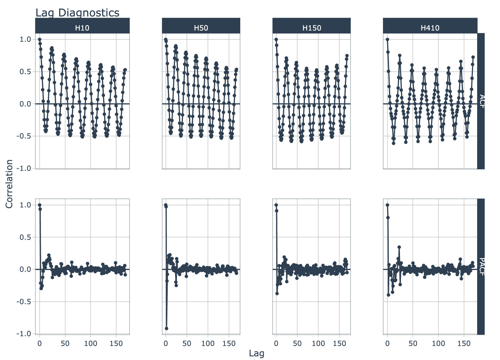
Grouped ACF Diagnostics
m4_hourly %>%
    group_by(id) %>%
    plot_acf_diagnostics(
        date, value,               # ACF & PACF
        .lags = "7 days",          # 7-Days of hourly lags
        .interactive = interactive
    )
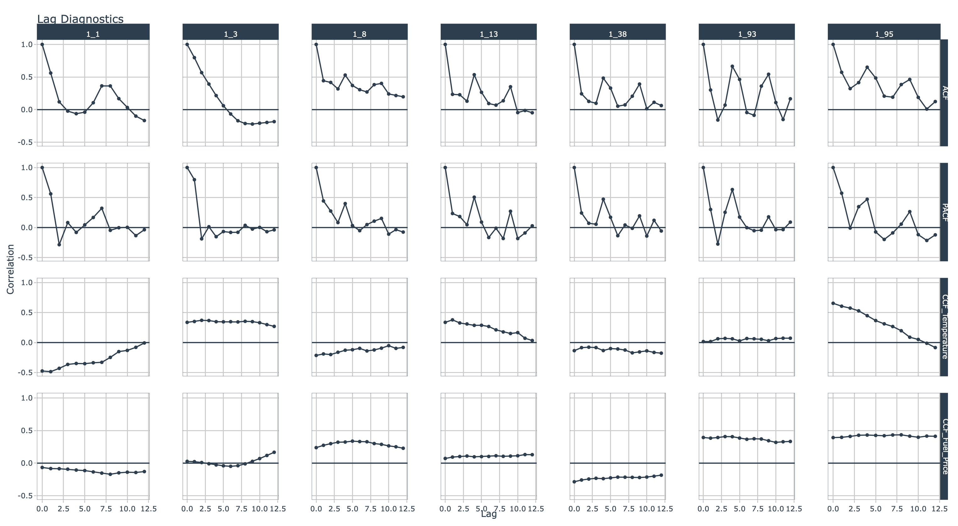
Grouped CCF Plots
walmart_sales_weekly %>%
    select(id, Date, Weekly_Sales, Temperature, Fuel_Price) %>%
    group_by(id) %>%
    plot_acf_diagnostics(
        Date, Weekly_Sales,        # ACF & PACF
        .ccf_vars    = c(Temperature, Fuel_Price),   # CCFs
        .lags        = "3 months",    # 3 months of weekly lags
        .interactive = interactive
    )
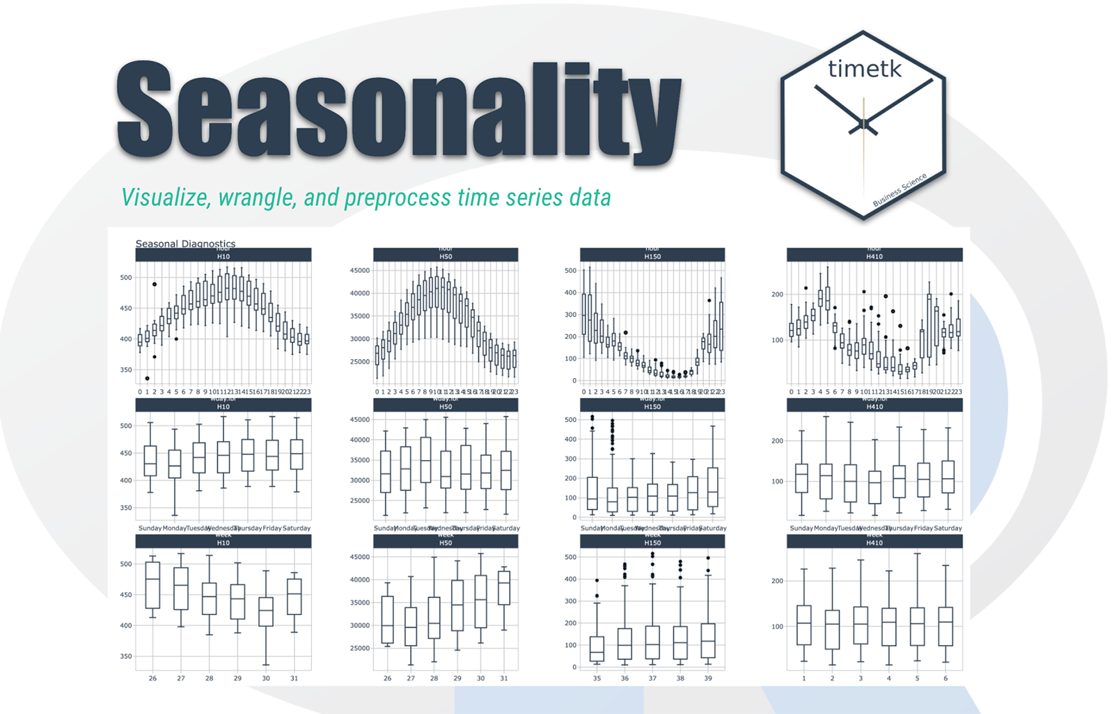
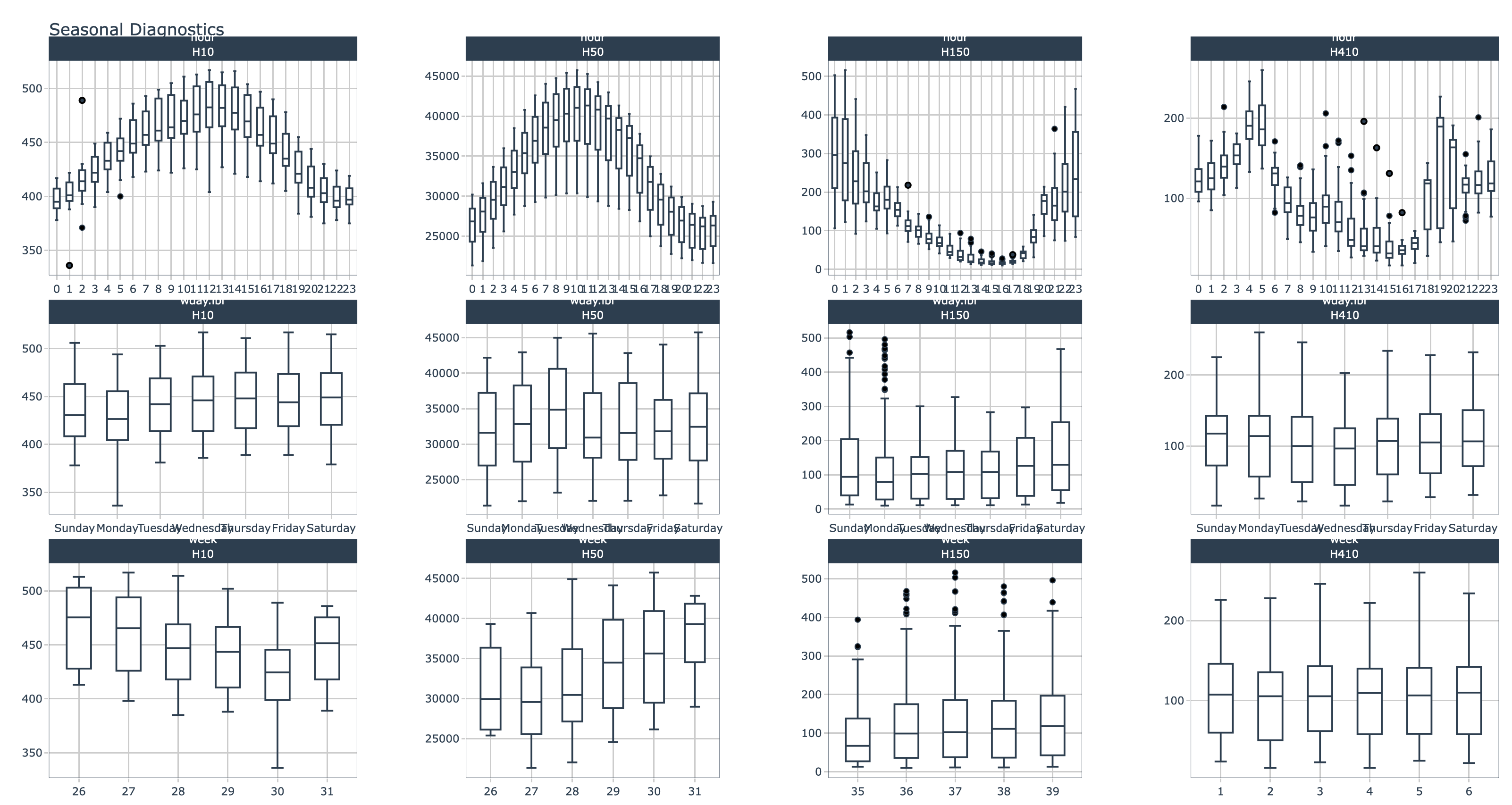
Seasonality
plot_seasonal_diagnostics() is an interactive and scalable function for visualizing time series seasonality.
Automatic Feature Selection
Internal calculations are performed to detect a sub-range of features to include using the following logic:
Example: Hourly timestamp data that lasts more than 2 weeks will have the following features: “hour”, “wday.lbl”, and “week”.
Scalable with Grouped Data Frames
This function respects grouped data.frame and tibbles that were made with dplyr::group_by().
For grouped data, the automatic feature selection returned is a collection of all features within the sub-groups. This means extra features are returned even though they may be meaningless for some of the groups.
The .value parameter respects transformations (e.g. .value = log(sales))
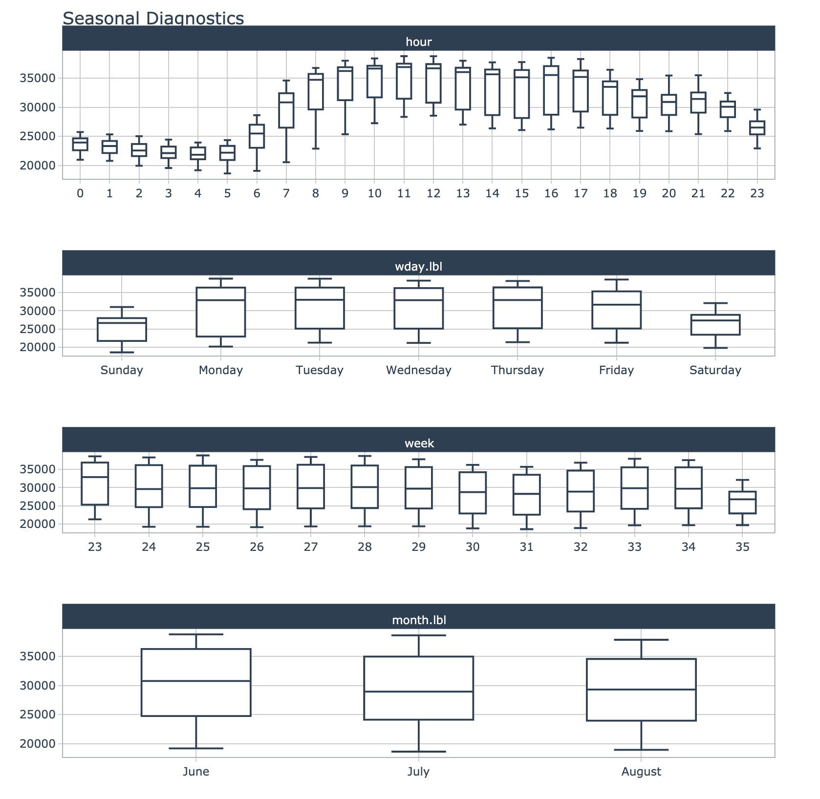
Seasonal Visualizations
taylor_30_min %>%
    plot_seasonal_diagnostics(date, value, .interactive = interactive)
Grouped Seasonal Visualizations
m4_hourly %>%
    group_by(id) %>%
    plot_seasonal_diagnostics(date, value, .interactive = interactive)
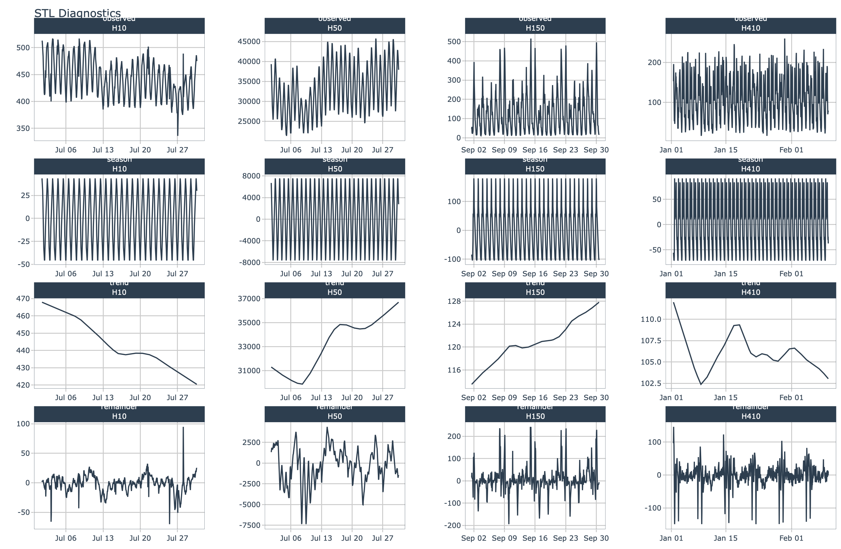
STL Diagnostics
The plot_stl_diagnostics() function generates a Seasonal-Trend-Loess decomposition. The function is “tidy” in the sense that it works on data frames and is designed to work with dplyr groups.
STL method
The STL method implements time series decomposition using the underlying stats::stl(). The decomposition separates the “season” and “trend” components from the “observed” values leaving the “remainder”.
Frequency & Trend Selection
The user can control two parameters: .frequency and .trend.
- The
.frequency parameter adjusts the “season” component that is removed from the “observed” values.
- The
.trend parameter adjusts the trend window (t.window parameter from stl()) that is used.
The user may supply both .frequency and .trend as time-based durations (e.g. “6 weeks”) or numeric values (e.g. 180) or “auto”, which automatically selects the frequency and/or trend based on the scale of the time series.
m4_hourly %>%
    group_by(id) %>%
    plot_stl_diagnostics(
        date, value,
        .frequency = "auto", .trend = "auto",
        .feature_set = c("observed", "season", "trend", "remainder"),
        .interactive = interactive)
Have questions on using Timetk for time series?
Make a comment in the chat below. 👇
And, if you plan on using timetk for your business, it’s a no-brainer - Join the Time Series Course.