Time Series in 5-Minutes, Part 1: Data Wrangling and Rolling Calculations
Written by Matt Dancho
Have 5-minutes? Then let’s learn time series. In this short articles series, I highlight how you can get up to speed quickly on important aspects of time series analysis. Today we are focusing preparing data for timeseries analysis rolling calculations.
Updates
This article has been updated. View the updated Time Series in 5-Minutes article at Business Science.
Time Series in 5-Mintues
Articles in this Series
Rolling Calculations - A fundamental tool in your arsenal
I just released timetk 2.0.0 (read the release announcement). A ton of new functionality has been added. We’ll discuss some of the key pieces in this article series:
👉 Register for our blog to get new articles as we release them.
Have 5-Minutes?
Then let’s learn Rolling Calculations
A collection of tools for working with time series in R
Time series data wrangling is an essential skill for any forecaster. timetk includes the essential data wrangling tools. In this tutorial:
- Summarise by Time - For time-based aggregations
- Filter by Time - For complex time-based filtering
- Pad by Time - For filling in gaps and going from low to high frequency
- Slidify - For turning any function into a sliding (rolling) function
Additional concepts covered:
- Imputation - Needed for Padding (See Low to High Frequency)
- Advanced Filtering - Using the new add time
%+time infix operation (See Padding Data: Low to High Frequency)
- Visualization -
plot_time_series() for all visualizations
Let’s Get Started
library(tidyverse)
library(tidyquant)
library(timetk)
Data
This tutorial will use the FANG dataset:
- Daily
- Irregular (missing business holidays and weekends)
- 4 groups (FB, AMZN, NFLX, and GOOG).
FANG
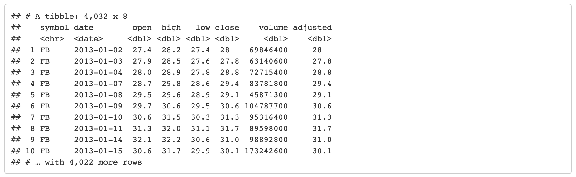
The adjusted column contains the adjusted closing prices for each day.
FANG %>%
  group_by(symbol) %>%
  plot_time_series(date, adjusted, .facet_ncol = 2, .interactive = FALSE)
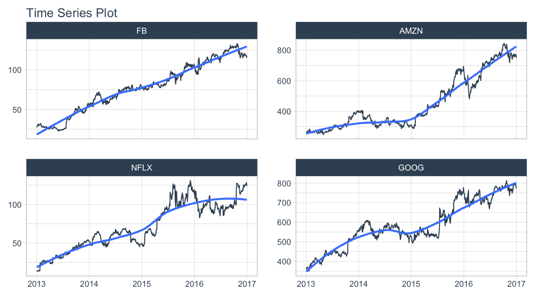
The volume column contains the trade volume (number of times the stock was transacted) for the day.
FANG %>%
  group_by(symbol) %>%
  plot_time_series(date, volume, .facet_ncol = 2, .interactive = FALSE)
Summarize by Time
summarise_by_time() aggregates by a period. It’s great for:
- Period Aggregation -
SUM()
- Period Smoothing -
AVERAGE(), FIRST(), LAST()
Period Summarization
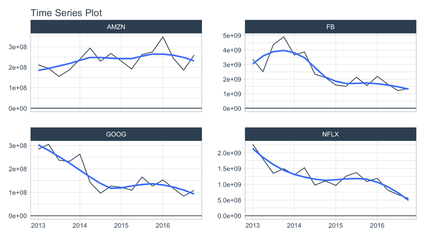
Objective: Get the total trade volume by quarter
- Use
SUM()
- Aggregate using
.by = "quarter"
FANG %>%
  group_by(symbol) %>%
  summarise_by_time(
    date, .by = "quarter",
    volume = SUM(volume)
  ) %>%
  plot_time_series(date, volume, .facet_ncol = 2, .interactive = FALSE, .y_intercept = 0)
Period Smoothing
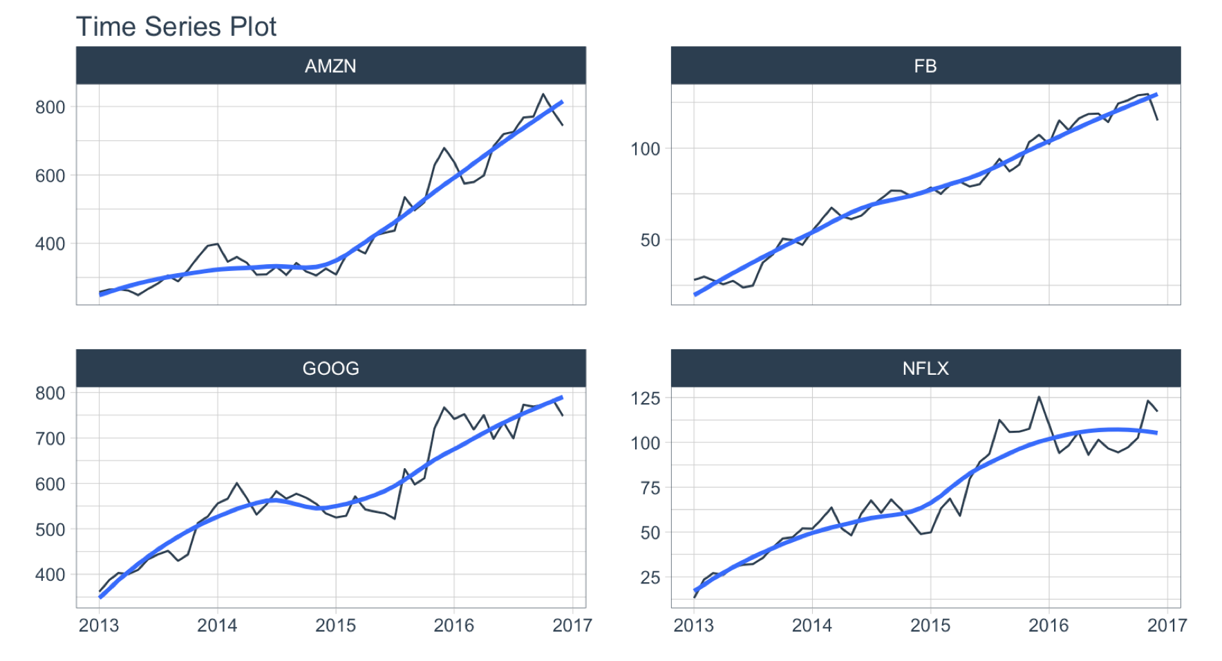
Objective: Get the first value in each month
- We can use
FIRST() to get the first value, which has the effect of reducing the data (i.e. smoothing). We could use AVERAGE() or MEDIAN().
- Use the summarization by time:
.by = "month" to aggregate by month.
FANG %>%
  group_by(symbol) %>%
  summarise_by_time(
    date, .by = "month",
    adjusted = FIRST(adjusted)
  ) %>%
  plot_time_series(date, adjusted, .facet_ncol = 2, .interactive = FALSE)
Filter By Time
Used to quickly filter a continuous time range.
Time Range Filtering
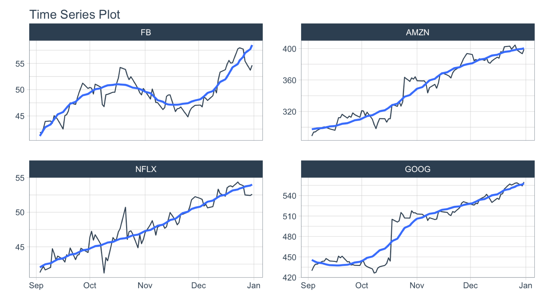
Objective: Get the adjusted stock prices in the 3rd quarter of 2013.
.start_date = "2013-09": Converts to “2013-09-01.end_date = "2013": Converts to “2013-12-31- A more advanced example of filtering using
%+time and %-time is shown in “Padding Data: Low to High Frequency”.
FANG %>%
  group_by(symbol) %>%
  filter_by_time(date, "2013-09", "2013") %>%
  plot_time_series(date, adjusted, .facet_ncol = 2, .interactive = FALSE)
Padding Data
Used to fill in (pad) gaps and to go from from low frequency to high frequency. This function uses the awesome padr library for filling and expanding timestamps.
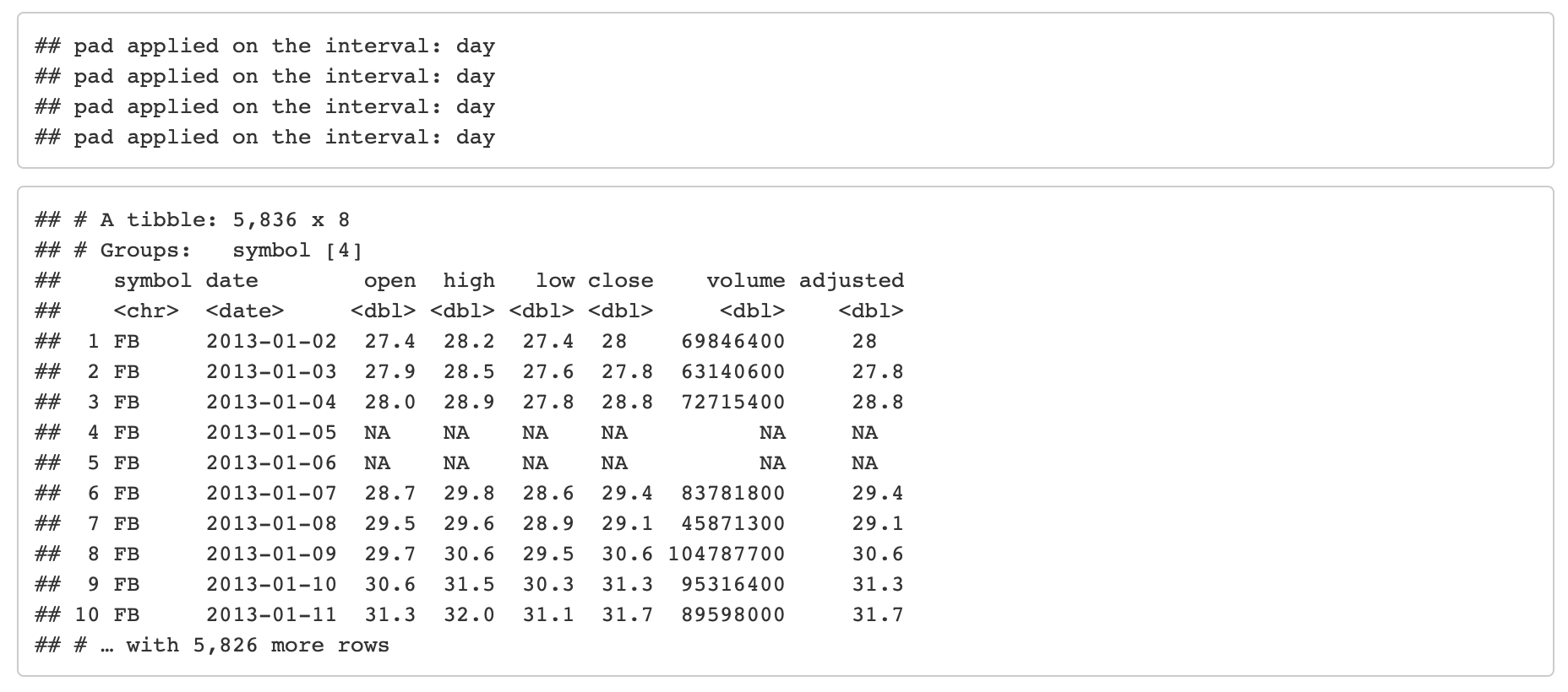
Fill in Gaps
Objective: Make an irregular series regular.
- We will leave padded values as
NA.
- We can add a value using
.pad_value or we can impute using a function like ts_impute_vec() (shown next).
FANG %>%
  group_by(symbol) %>%
  pad_by_time(date, .by = "auto") # Guesses .by = "day"
Low to High Frequency
Objective: Go from Daily to Hourly timestamp intervals for 1 month from the start date. Impute the missing values.
.by = "hour" pads from daily to hourly- Imputation of hourly data is accomplished with
ts_impute_vec(), which performs linear interpolation when period = 1.
- Filtering is accomplished using:
- “start”: A special keyword that signals the start of a series
FIRST(date) %+time% "1 month": Selecting the first date in the sequence then using a special infix operation, %+time%, called “add time”. In this case I add “1 month”.
FANG %>%
  group_by(symbol) %>%
  pad_by_time(date, .by = "hour") %>%
  mutate_at(vars(open:adjusted), .funs = ts_impute_vec, period = 1) %>%
  filter_by_time(date, "start", FIRST(date) %+time% "1 month") %>%
  plot_time_series(date, adjusted, .facet_ncol = 2, .interactive = FALSE)
Sliding (Rolling) Calculations
We have a new function, slidify() that turns any function into a sliding (rolling) window function. It takes concepts from tibbletime::rollify() and it improves them with the R package slider.
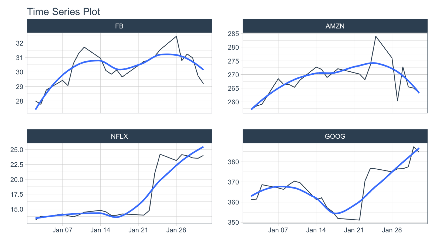
Rolling Mean
Objective: Calculate a “centered” simple rolling average with partial window rolling and the start and end windows.
slidify() turns the AVERAGE() function into a rolling average.
# Make the rolling function
roll_avg_30 <- slidify(.f = AVERAGE, .period = 30, .align = "center", .partial = TRUE)
# Apply the rolling function
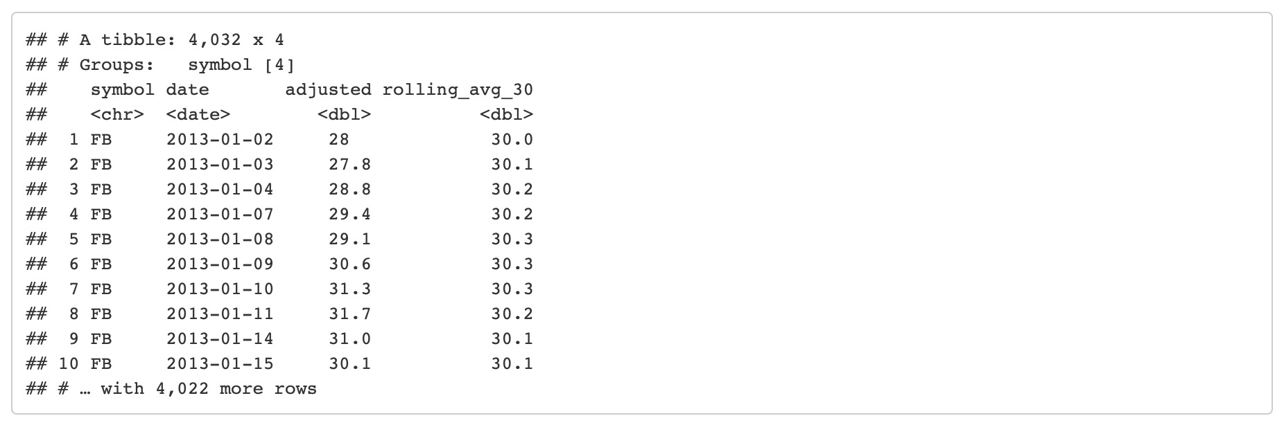
FANG %>%
select(symbol, date, adjusted) %>%
group_by(symbol) %>%
# Apply Sliding Function
mutate(rolling_avg_30 = roll_avg_30(adjusted)) %>%
pivot_longer(cols = c(adjusted, rolling_avg_30)) %>%
plot_time_series(date, value, .color_var = name,
.facet_ncol = 2, .smooth = FALSE,
.interactive = FALSE)
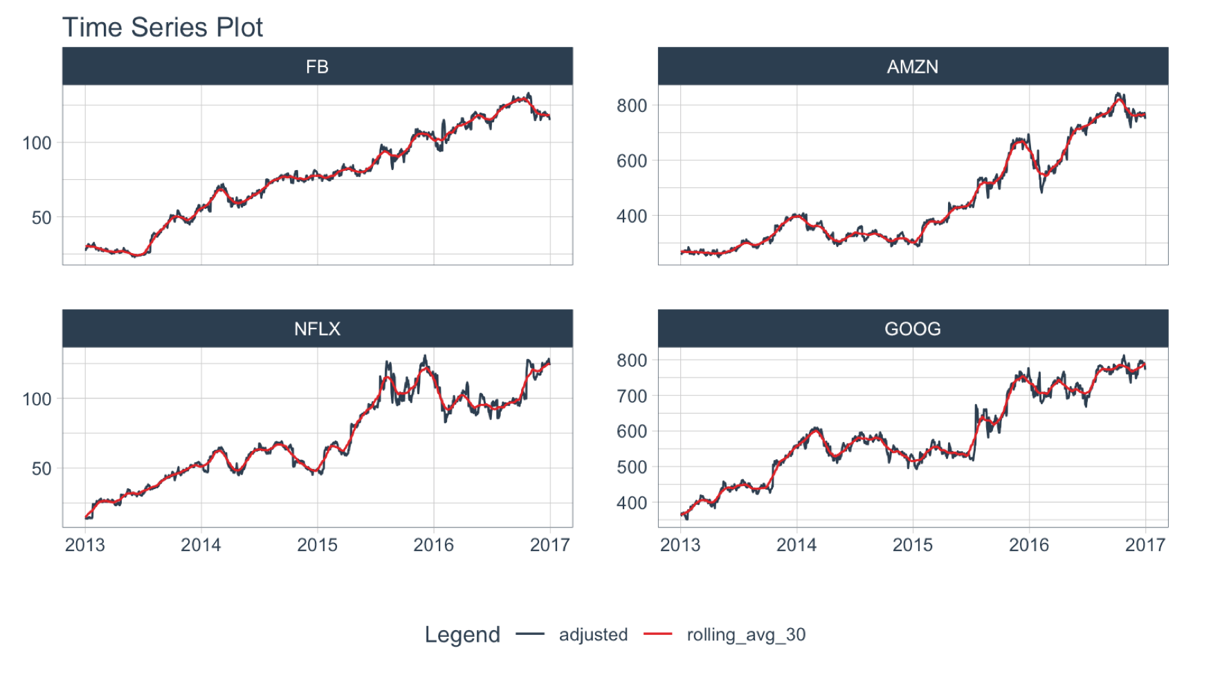
For simple rolling calculations (rolling average), we can accomplish this operation faster with slidify_vec() - A vectorized rolling function for simple summary rolls (e.g. mean(), sd(), sum(), etc)
FANG %>%
  select(symbol, date, adjusted) %>%
  group_by(symbol) %>%
  # Apply roll apply Function
  mutate(rolling_avg_30 = slidify_vec(adjusted,  ~ AVERAGE(.),
                                      .period = 30, .partial = TRUE))
Rolling Regression
Objective: Calculate a rolling regression.
- This is a complex sliding (rolling) calculation that requires multiple columns to be involved.
slidify() is built for this.- Use the multi-variable
purrr ..1, ..2, ..3, etc notation to setup a function
# Rolling regressions are easy to implement using `.unlist = FALSE`
lm_roll <- slidify(~ lm(..1 ~ ..2 + ..3), .period = 90,
.unlist = FALSE, .align = "right")
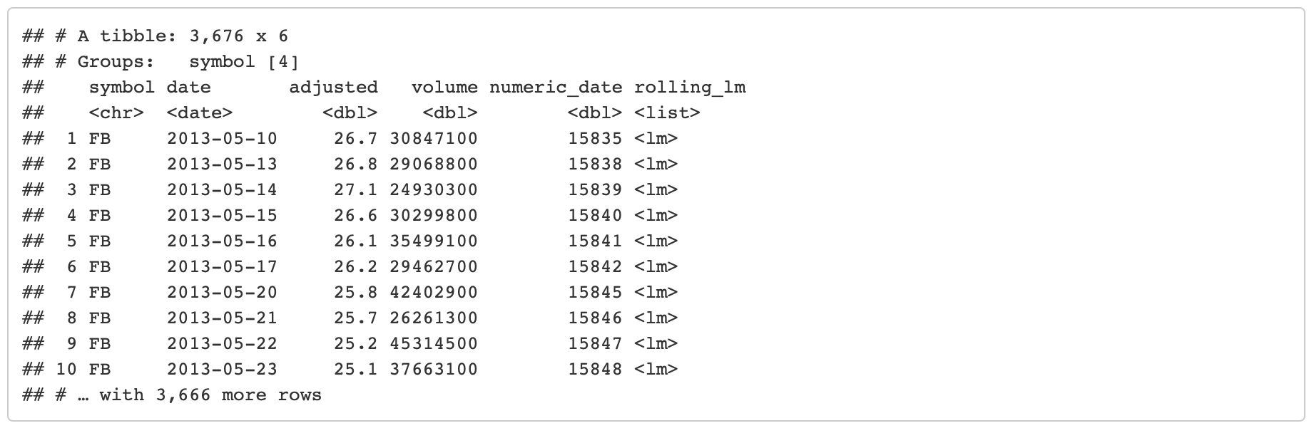
FANG %>%
select(symbol, date, adjusted, volume) %>%
group_by(symbol) %>%
mutate(numeric_date = as.numeric(date)) %>%
# Apply rolling regression
mutate(rolling_lm = lm_roll(adjusted, volume, numeric_date)) %>%
filter(!is.na(rolling_lm))
Have questions on using Timetk for time series?
Make a comment in the chat below. 👇
And, if you plan on using timetk for your business, it’s a no-brainer - Join the Time Series Course.