PDF Scraping in R with tabulizer
Written by Jennifer Cooper
This article comes from Jennifer Cooper, a new student in Business Science University. Jennifer is 35% complete with the 101 course - and shows off her progress in this PDF Scraping tutorial. Jennifer has an interest in understanding the plight of wildlife across the world, and uses her new data science skills to perform a useful analysis - scraping PDF tables of a Report on Endangered Species with the tabulizer R package and visualizing alarming trends with ggplot2.
R Packages Covered:
tabulizer - Scraping PDF tablesdplyr - Wrangling unclean data & preparation for data visualizationggplot2 - Data visualization and understanding trends
Scraping PDFs and Analyzing Endangered Species
Hey, everybody! Hope everyone has had a great weekend 😀!!
I’ve been “heads down” this weekend working on a special R project. This week I gave myself a challenge to start using R at work and also come up with a project on the side that I could use to help review what I’ve learned so far in Business Science University’s DS4B 101-R course.
In addition to being passionate about data science, I also love animals and am concerned about the plight of wildlife across the world, particularly with climate change. I decided to take a look at data on critically endangered species.
The only information on Endangered Species I could find was in a PDF format, so I spent a lot of time trying to figure out the nuances of tabulizer for scraping PDF. I finally got it done tonight!
Through this process, I discovered I still need a lot more practice, so I’m going to continue seeing what I can do to apply it at work (figure out how to connect to our SQL database this week), carve out more time to practice, and I may write up an article on working with tabulizer and PDFs.
Interested in learning R? Join me in the 101 course.
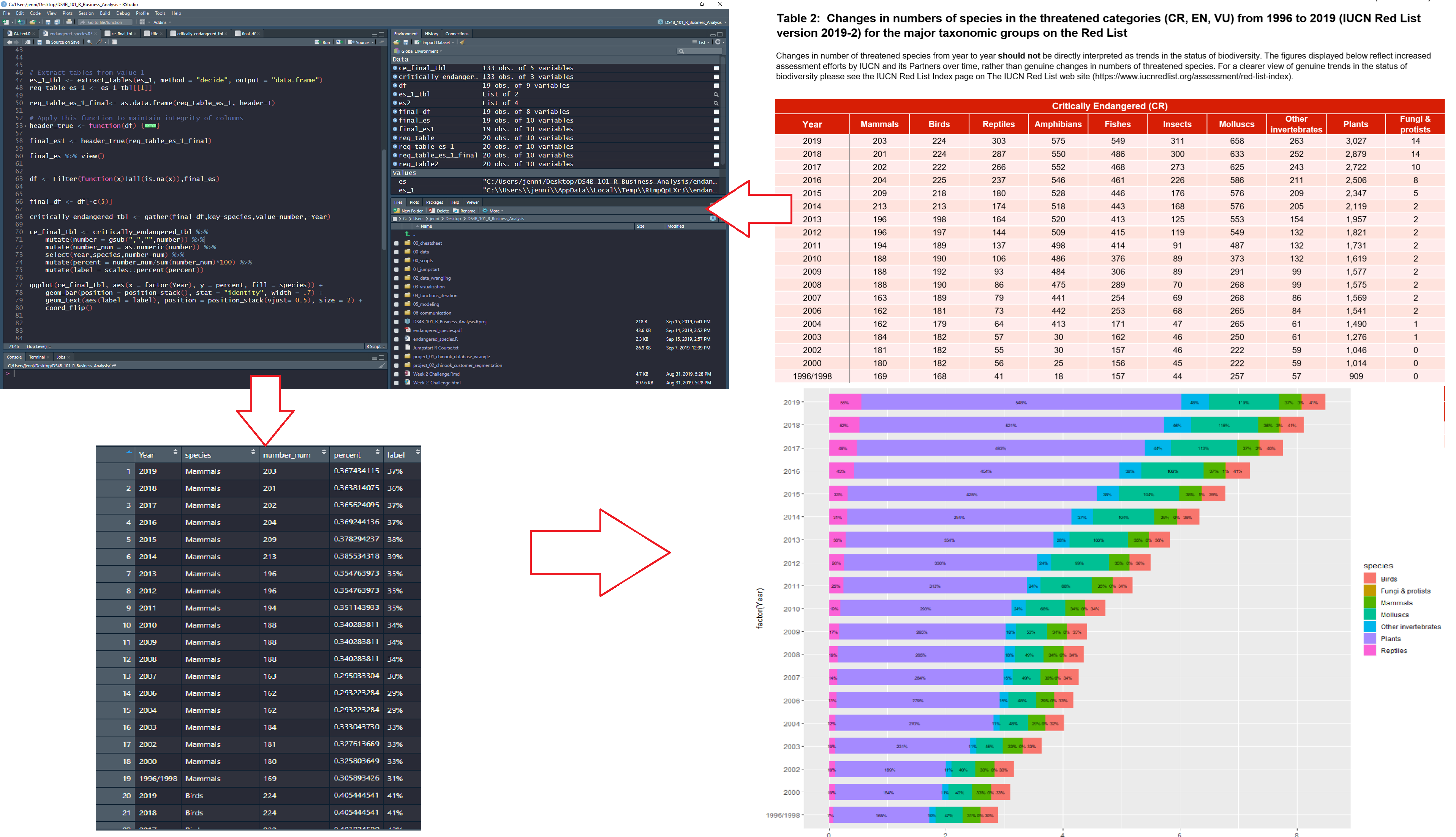
My Workflow
Here’s a diagram of the workflow I used:
-
Start with PDF
-
Use tabulizer to extract tables
-
Clean up data into “tidy” format using tidyverse (mainly dplyr)
-
Visualize trends with ggplot2
My Code Workflow for PDF Scraping with tabulizer
Get the PDF
I analyzed the Critically Endangered Species PDF Report.
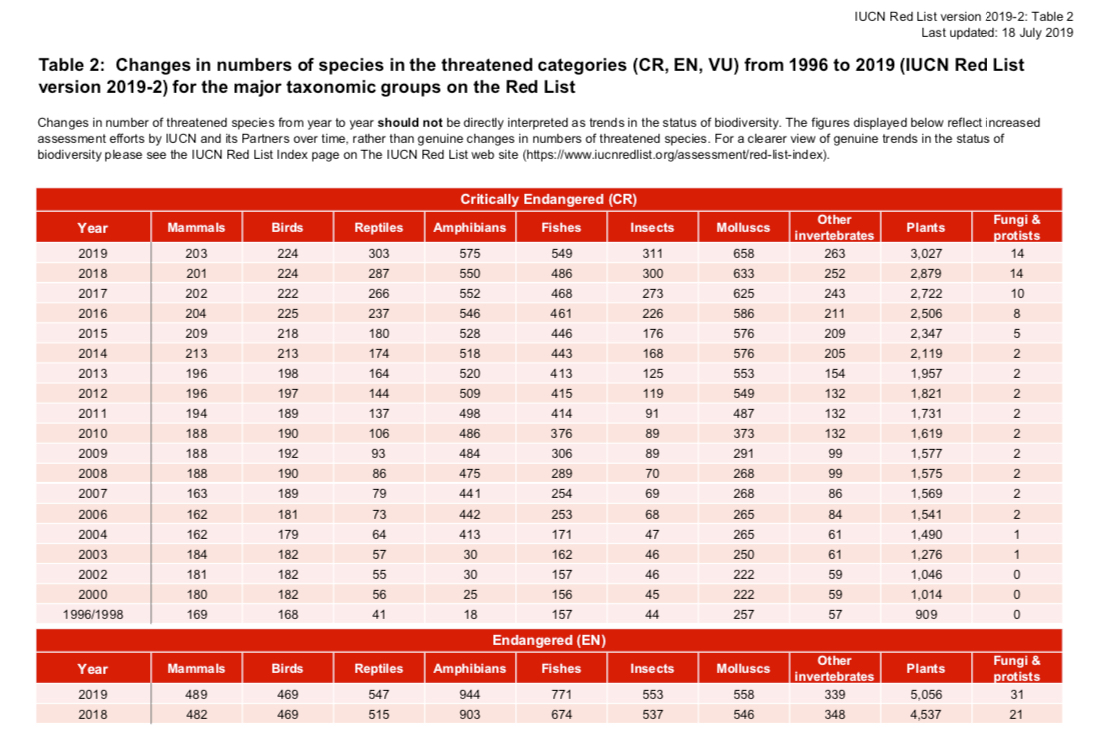
Get the Endangered Species PDF Report
PDF Scrape and Exploratory Analysis
Step 1 - Load Libraries
Load the following libraries to follow along.
library(rJava)      # Needed for tabulizer
library(tabulizer)  # Handy tool for PDF Scraping
library(tidyverse)  # Core data manipulation and visualization libraries
Note that tabulizer depends on rJava, which may require some setup. Here are a few pointers:
-
Mac Users: If you have issues connecting Java to R, you can try running sudo R CMD javareconf in the Terminal (per this post)
-
Windows Users: This blog article provides a step-by-step process for installing rJava on Windows machines.
The tabulizer package provides a suite of tools for extracting data from PDFs. The vignette, “Introduction to tabulizer” has a great overview of tabulizer’s features.
We’ll use the extract_tables() function to pull out each of the tables from the Endangered Species Report. This returns a list of data.frames.
# PDF Scrape Tables
endangered_species_scrape <- extract_tables(
    file   = "2019-09-23-tabulizer/endangered_species.pdf",
    method = "decide",
    output = "data.frame")
The table I’m interested in is the first one - the Critically Endangered Species. I’ll extract it using the pluck() function and convert it to a tibble() (the tidy data frame format). I see that I’m going to need to do a bit of cleanup.
# Pluck the first table in the list
endangered_species_raw_tbl <- endangered_species_scrape %>%
    pluck(1) %>%
    as_tibble()

# Show first 6 rows
endangered_species_raw_tbl %>% head() %>% knitr::kable()
| X |
X.1 |
X.2 |
X.3 |
Critically.Endangered..CR. |
X.4 |
X.5 |
X.6 |
X.7 |
X.8 |
| Year |
Mammals |
Birds |
Reptiles |
Amphibians Fishes Insects |
Molluscs |
Other invertebrates |
NA |
Plants |
Fungi & protists |
| 2019 |
203 |
224 |
303 |
575 549 311 |
658 |
263 |
NA |
3,027 |
14 |
| 2018 |
201 |
224 |
287 |
550 486 300 |
633 |
252 |
NA |
2,879 |
14 |
| 2017 |
202 |
222 |
266 |
552 468 273 |
625 |
243 |
NA |
2,722 |
10 |
| 2016 |
204 |
225 |
237 |
546 461 226 |
586 |
211 |
NA |
2,506 |
8 |
| 2015 |
209 |
218 |
180 |
528 446 176 |
576 |
209 |
NA |
2,347 |
5 |
Step 3 - Clean Up Column Names
Next, I want to start by cleaning up the names in my data - which are actually in the first row. I’ll use a trick using slice() to grab the first row, and the new pivot_longer() function to transpose and extract the column names that are in row 1. I can then set_names() and remove row 1.
# Get column names from Row 1
col_names <- endangered_species_raw_tbl %>%
    slice(1) %>%
    pivot_longer(cols = everything()) %>%
    mutate(value = ifelse(is.na(value), "Missing", value)) %>%
    pull(value)

# Overwrite names and remove Row 1
endangered_species_renamed_tbl <- endangered_species_raw_tbl %>%
    set_names(col_names) %>%
    slice(-1)

# Show first 6 rows
endangered_species_renamed_tbl %>% head() %>% knitr::kable()
| Year |
Mammals |
Birds |
Reptiles |
Amphibians Fishes Insects |
Molluscs |
Other invertebrates |
Missing |
Plants |
Fungi & protists |
| 2019 |
203 |
224 |
303 |
575 549 311 |
658 |
263 |
NA |
3,027 |
14 |
| 2018 |
201 |
224 |
287 |
550 486 300 |
633 |
252 |
NA |
2,879 |
14 |
| 2017 |
202 |
222 |
266 |
552 468 273 |
625 |
243 |
NA |
2,722 |
10 |
| 2016 |
204 |
225 |
237 |
546 461 226 |
586 |
211 |
NA |
2,506 |
8 |
| 2015 |
209 |
218 |
180 |
528 446 176 |
576 |
209 |
NA |
2,347 |
5 |
| 2014 |
213 |
213 |
174 |
518 443 168 |
576 |
205 |
NA |
2,119 |
2 |
Step 4 - Tidy the Data
There are a few issues with the data:
-
Remove columns with NAs: Column labelled “Missing” is all NA’s - We can just drop this column
-
Fix columns that were combined: Three of the columns are combined - Amphibians, Fishes, and Insects - We can separate() these into 3 columns
-
Convert to (Tidy) Long Format for visualization: The data is in “wide” format, which isn’t tidy - We can use pivot_longer() to convert to “long” format with one observation for each row
-
Fix numeric data stored as character: The numeric data is stored as character and several of the numbers have commas - We’ll remove commas and convert to numeric
-
Convert Character Year & species to Factor: The year and species columns are character - We can convert to factor for easier adjusting of the order in the ggplot2 visualizations
-
Percents by year: The visualizations will have a percent (proportion) included so we can see which species have the most endangered - We can add proportions by each year
endangered_species_final_tbl <- endangered_species_renamed_tbl %>%

    # 1. Remove columns with NAs
    select_if(~ !all(is.na(.))) %>%

    # 2. Fix columns that were combined
    separate(col  = `Amphibians Fishes Insects`,
             into = c("Amphibians", "Fishes", "Insects"),
             sep  = " ") %>%

    # 3. Convert to (Tidy) Long Format for visualization
    pivot_longer(cols = -Year, names_to = "species", values_to = "number") %>%

    # 4. Fix numeric data stored as character
    mutate(number = str_remove_all(number, ",")) %>%
    mutate(number = as.numeric(number)) %>%

    # 5. Convert Character Year & species to Factor
    mutate(Year = as_factor(Year)) %>%
    mutate(species = as.factor(species)) %>%

    # 6. Percents by year
    group_by(Year) %>%
    mutate(percent = number / sum(number)) %>%
    mutate(label = scales::percent(percent)) %>%
    ungroup()

# Show first 6 rows
endangered_species_final_tbl %>% head() %>% knitr::kable()
| Year |
species |
number |
percent |
label |
| 2019 |
Mammals |
203 |
0.0331320 |
3.3% |
| 2019 |
Birds |
224 |
0.0365595 |
3.7% |
| 2019 |
Reptiles |
303 |
0.0494532 |
4.9% |
| 2019 |
Amphibians |
575 |
0.0938469 |
9.4% |
| 2019 |
Fishes |
549 |
0.0896034 |
9.0% |
| 2019 |
Insects |
311 |
0.0507589 |
5.1% |
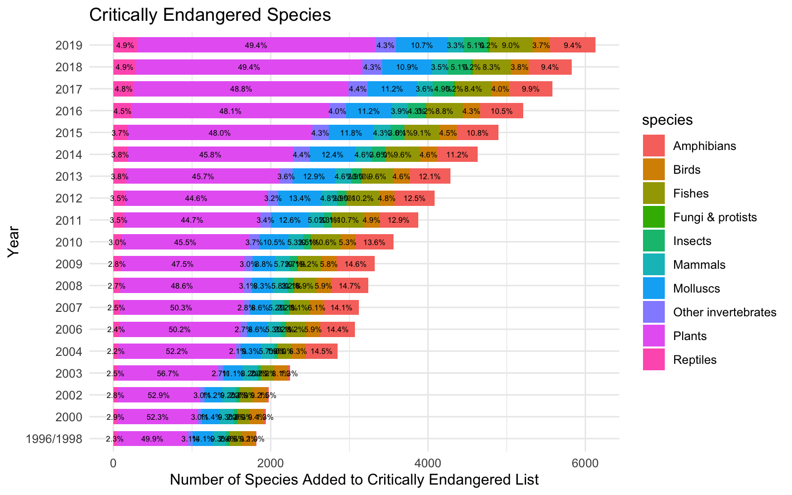
Step 5 - Visualize the Data
Summary Visualization
I made a summary visualization using stacked bar chart to show the alarming trends of critically endangered species over time.
endangered_species_final_tbl %>%
    mutate(Year = fct_rev(Year)) %>%

    ggplot(aes(x = Year, y = number, fill = species)) +

    # Geoms
    geom_bar(position = position_stack(), stat = "identity", width = .7) +
    geom_text(aes(label = label), position = position_stack(vjust= 0.5), size = 2) +
    coord_flip() +

    # Theme
    labs(
        title = "Critically Endangered Species",
        y = "Number of Species Added to Critically Endangered List", x = "Year"
    ) +
    theme_minimal()
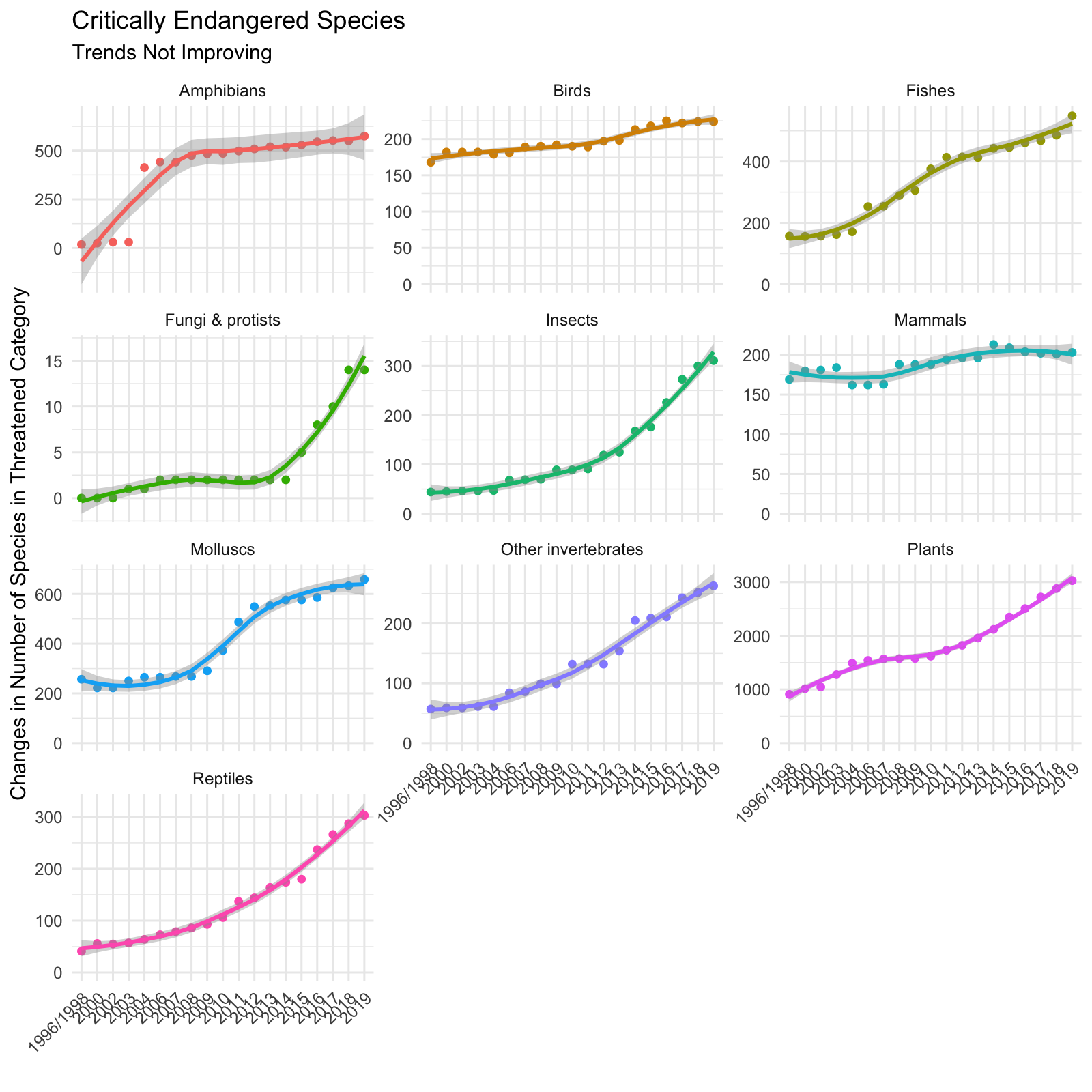
Trends Over Time by Species
I then faceted the species and visualized the trend over time using a smoother (geom_smooth). Again, we see that each of the species exhibit increasing trends.
endangered_species_final_tbl %>%
    mutate(Year = fct_rev(Year)) %>%

    # Geom
    ggplot(aes(Year, number, color = species, group = species)) +
    geom_point() +
    geom_smooth(method = "loess") +
    facet_wrap(~ species, scales = "free_y", ncol = 3) +

    # Theme
    expand_limits(y = 0) +
    theme_minimal() +
    theme(legend.position = "none",
          axis.text.x = element_text(angle = 45, hjust = 1)) +
    labs(
        title = "Critically Endangered Species",
        subtitle = "Trends Not Improving",
        x = "", y = "Changes in Number of Species in Threatened Category"
    )
Parting Thoughts
It was really exciting to see my hard work pay off. It took a bit to get going, but I found that tabulizer made PDF extraction manageable. The most challenging part was getting the data into a format that can be easily visualized (the tidyverse really helped as shown in Step 4!). I was particularly excited to see results of my analysis. I want to share with others the alarming trends related to the plight of wildlife, while demonstrating the power of R!
If you’d like to join me, I’m currently learning Data Science for Business in Business Science’s 101 course (Data Science Foundations), and I’ve signed up for 201 Advanced Machine Learning and 102 Shiny Web Applications.
See what our students are doing:
Student Success Stories
Real stories of success from our students applying their skills learned at Business Science University to get jobs and help their organizations!
Student Code Tutorials
Tutorials made by our students using their new skills learned at Business Science University!