Cleaning Anomalies to Reduce Forecast Error by 9% with anomalize
Written by Matt Dancho
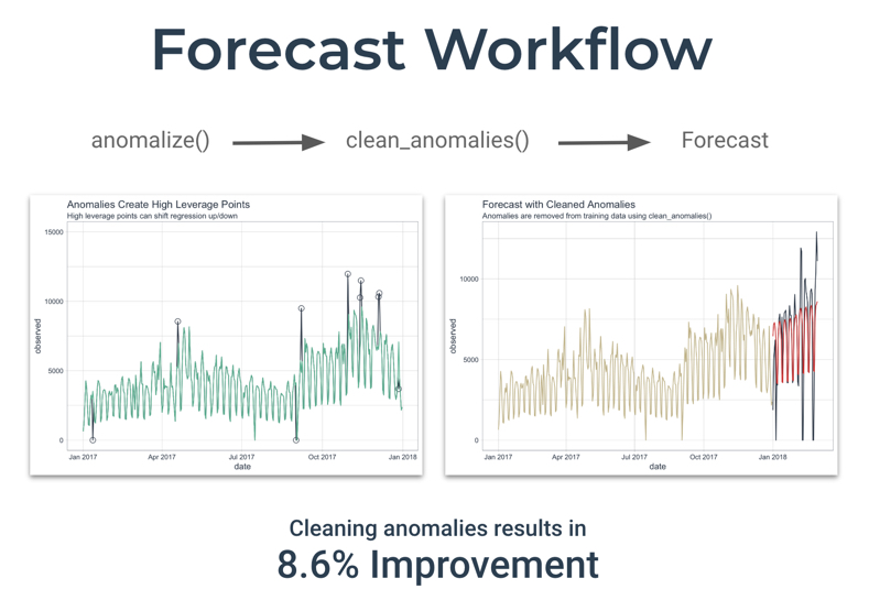
In this tutorial, we’ll show how we used clean_anomalies() from the anomalize package to reduce forecast error by 9%.
R Packages Covered:
anomalize - Time series anomaly detection
Cleaning Anomalies to Reduce Forecast Error by 9%
We can often improve forecast performance by cleaning anomalous data prior to forecasting. This is the perfect use case for integrating the clean_anomalies() function from anomalize into your forecast workflow.
Forecast Workflow

We’ll use the following workflow to remove time series anomalies prior to forecasting.
-
Identify the anomalies - Decompose the time series with time_decompose() and anomalize() the remainder (residuals)
-
Clean the anomalies - Use the new clean_anomalies() function to reconstruct the time series, replacing anomalies with the trend and seasonal components
-
Forecast - Use a forecasting algorithm to predict new observations from a training set, then compare to test set with and without anomalies cleaned
Step 1 - Load Libraries
First, load the following libraries to follow along.
library(tidyverse)  # Core data manipulation and visualization libraries
library(tidyquant)  # Used for business-ready ggplot themes
library(anomalize)  # Identify and clean time series anomalies
library(timetk)     # Time Series Machine Learning Features
library(knitr)      # For kable() function
Step 2 - Get the Data
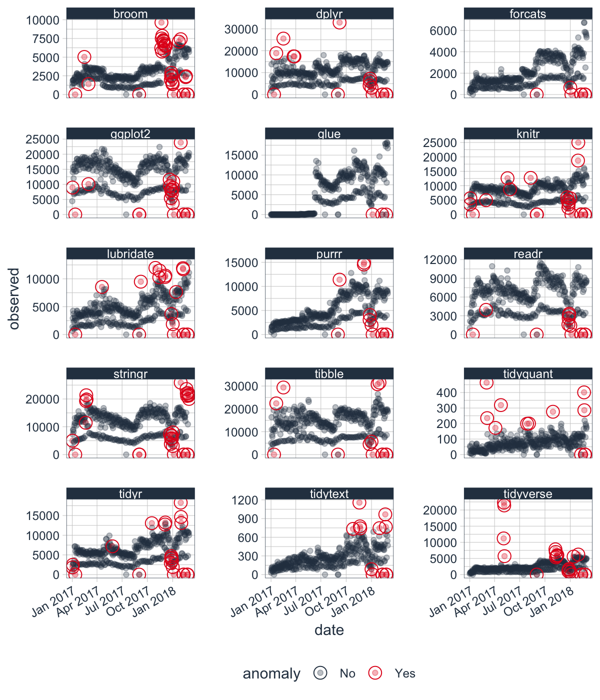
This tutorial uses the tidyverse_cran_downloads dataset that comes with anomalize. These are the historical downloads of several “tidy” R packages from 2017-01-01 to 2018-03-01.
Let’s take one package with some extreme events. We’ll hone in on lubridate (but you could pick any).
tidyverse_cran_downloads %>%
    time_decompose(count) %>%
    anomalize(remainder) %>%
    time_recompose() %>%
    plot_anomalies(ncol = 3, alpha_dots = 0.3)
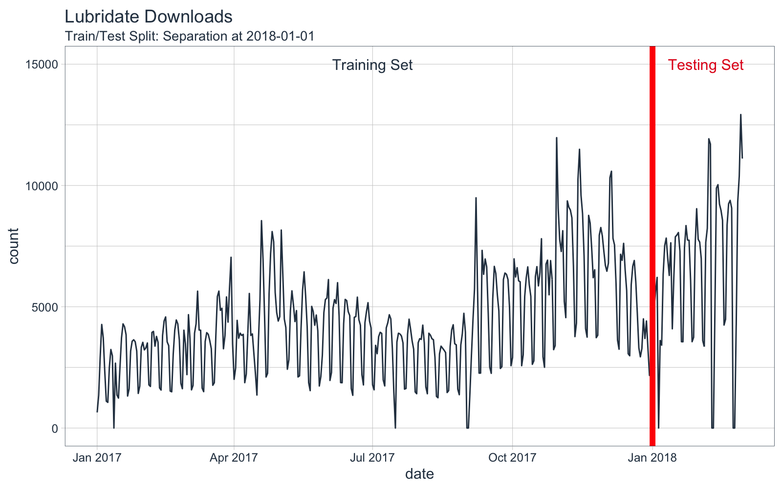
We’ll filter() downloads of the lubridate R package.
lubridate_tbl <- tidyverse_cran_downloads %>%
  ungroup() %>%
  filter(package == "lubridate")
Here’s a visual representation of the forecast experiment setup. Training data will be any data before “2018-01-01”.
Step 3 - Workflow for Cleaning Anomalies
The workflow to clean anomalies:
-
We decompose the “counts” column using time_decompose() - This returns a Seasonal-Trend-Loess (STL) Decomposition in the form of “observed”, “season”, “trend” and “remainder”.
-
We fix any negative values - If present, they can throw off forecasting transformations (e.g. log and power transformations)
-
We identifying anomalies (anomalize()) on the “remainder” column - Returns “remainder_l1” (lower limit), “remainder_l2” (upper limit), and “anomaly” (Yes/No).
-
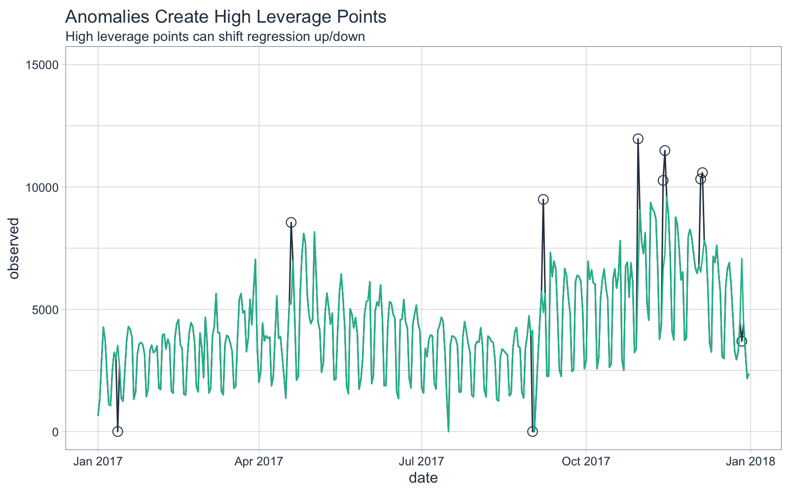
We use the function, clean_anomalies(), to add new column called “observed_cleaned” that repairs the anomalous data by replacing all anomalies with the trend + seasonal components from the decompose operation.
lubridate_anomalized_tbl <- lubridate_tbl %>%

    # 1. Decompose download counts and anomalize the STL decomposition remainder
    time_decompose(count) %>%

    # 2. Fix negative values if any in observed
    mutate(observed = ifelse(observed < 0, 0, observed)) %>%

    # 3. Identify anomalies
    anomalize(remainder) %>%

    # 4. Clean & repair anomalous data
    clean_anomalies()

# Show change in observed vs observed_cleaned
lubridate_anomalized_tbl %>%
  filter(anomaly == "Yes") %>%
  select(date, anomaly, observed, observed_cleaned) %>%
  head() %>%
  kable()
| date |
anomaly |
observed |
observed_cleaned |
| 2017-01-12 |
Yes |
0 |
3522.194 |
| 2017-04-19 |
Yes |
8549 |
5201.716 |
| 2017-09-01 |
Yes |
0 |
4136.721 |
| 2017-09-07 |
Yes |
9491 |
4871.176 |
| 2017-10-30 |
Yes |
11970 |
6412.571 |
| 2017-11-13 |
Yes |
10267 |
6640.871 |
Here’s a visual of the “observed” (uncleaned) vs the “observed_cleaned” (cleaned) training sets. We’ll see what influence these anomalies have on a forecast regression (next).
Step 4 - Forecasting Downloads of the Lubridate Package
First, we’ll make a function, forecast_downloads(), that can take the input of both cleaned and uncleaned anomalies and return the forecasted downloads versus actual downloads. The modeling function is described in the Appendix - Forecast Downloads Function.
Step 4.1 - Before Cleaning with anomalize
We’ll first perform a forecast without cleaning anomalies (high leverage points).
- The
forecast_downloads() function trains on the “observed” (uncleaned) data and returns predictions versus actual.
- Internally, a power transformation (square-root) is applied to improve the forecast due to the multiplicative properties.
- The model uses a linear regression of the form
sqrt(observed) ~ numeric index + year + quarter + month + day of week.
lubridate_forecast_with_anomalies_tbl <- lubridate_anomalized_tbl %>%

    # See Apendix - Forecast Downloads Function
    forecast_downloads(
        col_train = observed,     # First train with anomalies included
        sep       = "2018-01-01", # Separate at 1st of year
        trans     = "sqrt"        # Perform sqrt() transformation
    )
Forecast vs Actual Values
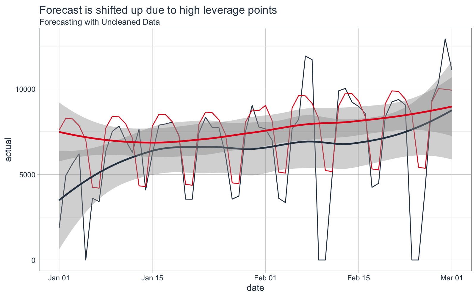
The forecast is overplotted against the actual values.
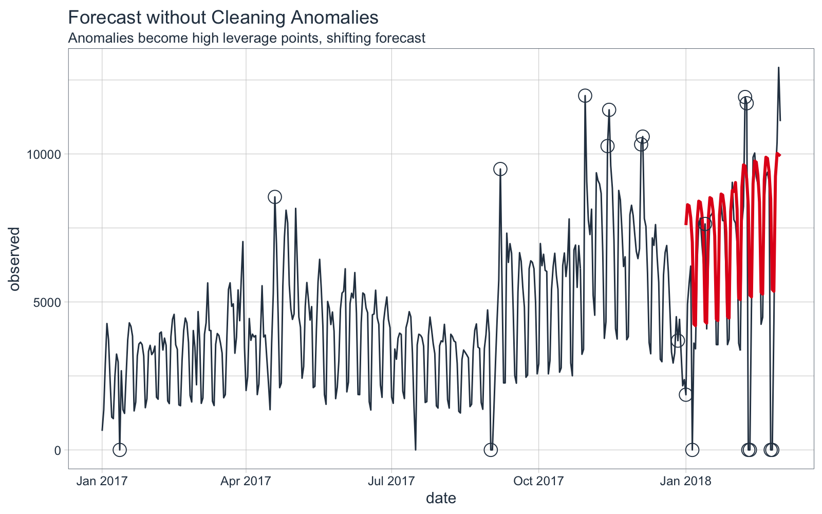
We can see that the forecast is shifted vertically, an effect of the high leverage points.
Forecast Error Calculation
The mean absolute error (MAE) is 1570, meaning on average the forecast is off by 1570 downloads each day.
lubridate_forecast_with_anomalies_tbl %>%
    summarise(mae = mean(abs(prediction - actual)))
## # A tibble: 1 x 1
##     mae
##   <dbl>
## 1 1570.
Step 4.2 - After Cleaning with anomalize
We’ll next perform a forecast this time using the repaired data from clean_anomalies().
- The
forecast_downloads() function trains on the “observed_cleaned” (cleaned) data and returns predictions versus actual.
- Internally, a power transformation (square-root) is applied to improve the forecast due to the multiplicative properties.
- The model uses a linear regression of the form
sqrt(observed_cleaned) ~ numeric index + year + quarter + month + day of week
lubridate_forecast_without_anomalies_tbl <- lubridate_anomalized_tbl %>%

    # See Appendix - Forecast Downloads Function
    forecast_downloads(
        col_train = observed_cleaned, # Forecast with cleaned anomalies
        sep       = "2018-01-01",     # Separate at 1st of year
        trans     = "sqrt"            # Perform sqrt() transformation
    )
Forecast vs Actual Values
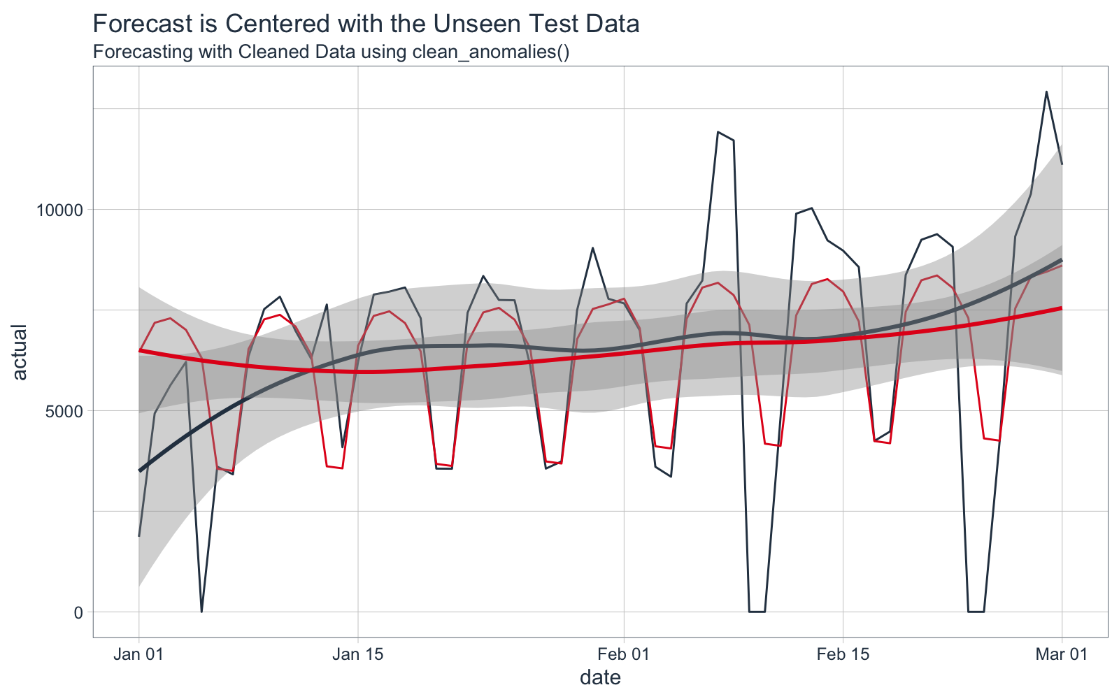
The forecast is overplotted against the actual values. The cleaned data is shown in Yellow.
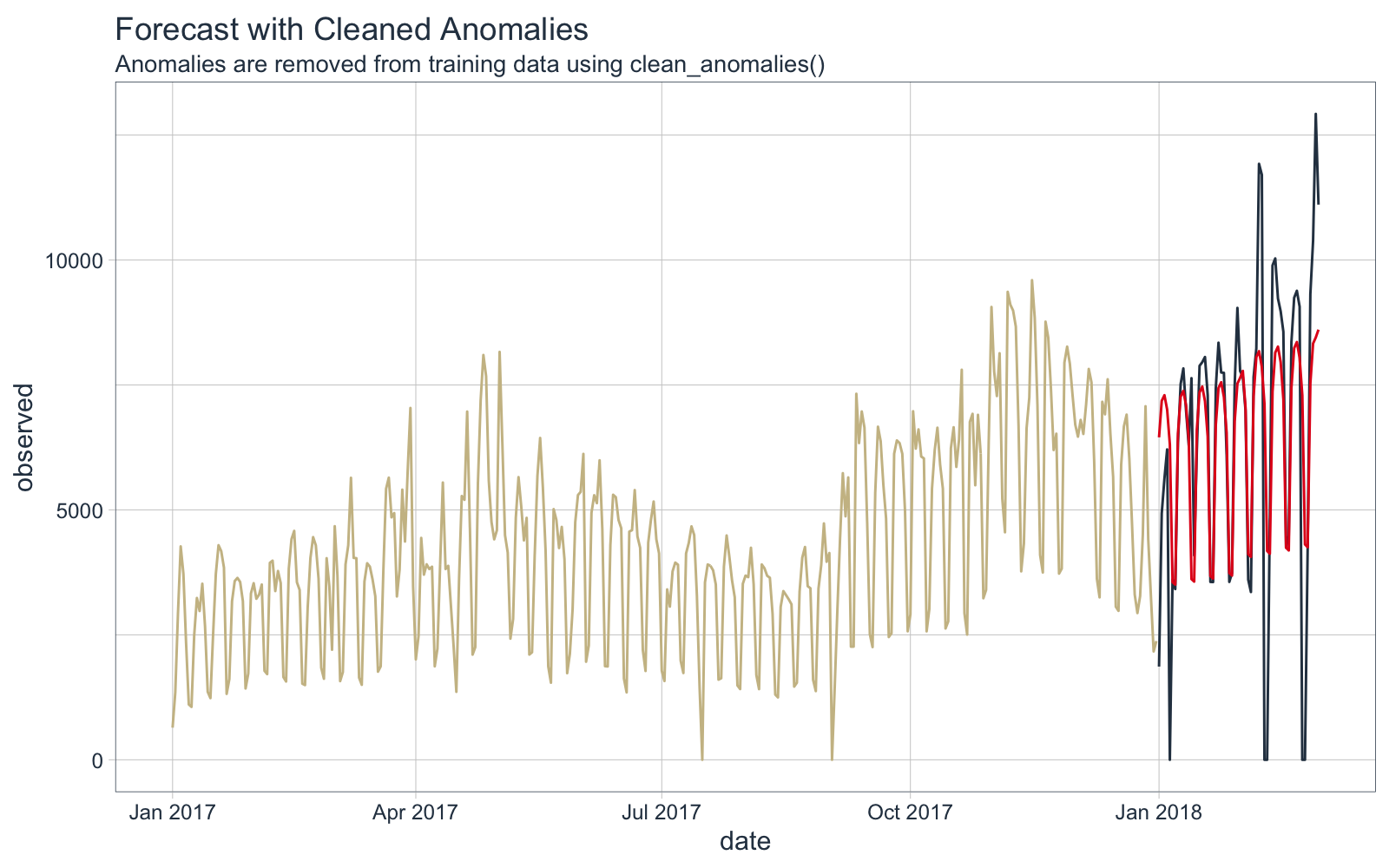
Zooming in on the forecast region, we can see that the forecast does a better job following the trend in the test data.
Forecast Error Calculation
The mean absolute error (MAE) is 1435, meaning on average the forecast is off by 1435 downloads each day.
lubridate_forecast_without_anomalies_tbl %>%
    summarise(mae = mean(abs(prediction - actual)))
## # A tibble: 1 x 1
##     mae
##   <dbl>
## 1 1435.
8.6% Reduction in Forecast Error
Using the new anomalize function, clean_anomalies(), prior to forecasting results in an 8.6% reduction in forecast error as measure by Mean Absolute Error (MAE).
((1435 - 1570) / 1570)
## [1] -0.08598726
Conclusion
Forecasting with clean anomalies is a good practice that can provide substantial improvement to forecasting accuracy by removing high leverage points. The new clean_anomalies() function in the anomalize package provides an easy workflow for removing anomalies prior to forecasting. Learn more in the anomalize documentation.
Data Science Training
Interested in Learning Anomaly Detection?
Business Science offers two 1-hour labs on Anomaly Detection:
Interested in Improving Your Forecasting?
Business Science offers a 1-hour lab on increasing Forecasting Accuracy:
- Learning Lab 5 - 5 Strategies to Improve Forecasting Performance by 50% (or more) using
arima and glmnet
Interested in Becoming an Expert in Data Science for Business?
Business Science offers a 3-Course Data Science for Business R-Track designed to take students from no experience to an expert data scientists (advanced machine learning and web application development) in under 6-months.
Appendix - Forecast Downloads Function
The forecast_downloads() function uses the following procedure:
- Split the
data into training and testing data using a date specified using the sep argument.
- Apply a statistical transformation: none, log-1-plus (
log1p()), or power (sqrt())
- Model the daily time series of the training data set from observed (demonstrates no cleaning) or observed and cleaned (demonstrates improvement from cleaning). Specified by the
col_train argument.
- Compares the predictions to the observed values.
forecast_downloads <- function(data, col_train,
                               sep = "2018-01-01",
                               trans = c("none", "log1p", "sqrt")) {


    predict_expr <- enquo(col_train)
    trans <- trans[1]

    # Spit into training/testing sets
    train_tbl <- data %>% filter(date < ymd(sep))
    test_tbl  <- data %>% filter(date >= ymd(sep))

    # Apply Transformation
    pred_form <- quo_name(predict_expr)
    if (trans != "none") pred_form <- str_glue("{trans}({pred_form})")

    # Make the model formula
    model_formula <- str_glue("{pred_form} ~ index.num + half
                              + quarter + month.lbl + wday.lbl") %>%
        as.formula()

    # Apply model formula to data that is augmented with time-based features
    model_glm <- train_tbl %>%
        tk_augment_timeseries_signature() %>%
        glm(model_formula, data = .)

    # Make Prediction
    suppressWarnings({
        # Suppress rank-deficit warning
        prediction <- predict(model_glm, newdata = test_tbl %>%
                                  tk_augment_timeseries_signature())
        actual     <- test_tbl %>% pull(!! actual_expr)
    })

    if (trans == "log1p") prediction <- expm1(prediction)
    if (trans == "sqrt")  prediction <- ifelse(prediction < 0, 0, prediction)^2

    # Return predictions and actual
    tibble(
        date       = tk_index(test_tbl),
        prediction = prediction,
        actual     = observed
    )
}