Excel to R, Part 1 - The 10X Productivity Boost
Written by Matt Dancho

Transitioning from Excel to R is one of the best decisions I have ever made. It accelerated my career and it boosted my productivity 10X - 100X (I show how in a Time Study - keep reading). I used Excel primarily for sales and marketing analytics. I was a power-user of Excel fully equipped in VBA, Pivot Tables, Conditional Formatting, and all the functions. I was really good.
So, why did I make the switch?

The short answer is that Excel has painful limitations. Excel grinds to a halt with “large” VLOOKUPS, often sitting idly with the spinning wheel or crashing computers as file sizes approach 50MB. Plus, I didn’t know it at the time, but I was very innefficient in my approach to analysis.
In a world where the data being generated was far exceeding my ability to analyze it in Excel (i.e. 50MB), I needed a better tool. The tool I went to was R - a free and open source tool that’s in high demand for many reasons - I discuss 6 reasons to use R for business in this article.
The bottom line is that learning R was an amazing decision, one that has changed my life. I’d like to share how to use R with you.
I learn best by following real-world applications, so this tutorial will follow a Marketing Case Study first showing the errors, limitations, and inefficiencies of Excel (Part 1) and next how to perform the marketing analysis in R (Parts 2 and 3).
If you learn best from real-world applications, then don’t miss the Business Science University Curriculum below - We have a fully integrated 3-Course R-Track that will help you advance your career. All of the tools in this article series are taught in the R-Track plus advanced Machine Learning and Shiny Web Apps using real-world applications.
Read this article series, to see how you can gain a 10X productivity boost by switching from Excel to R!
Articles in this Series
Part 1 Overview

Bank of America Term Deposits
In this 3-part series on Excel to R, we’ll follow a Marketing Case Study for a bank that has a product (Term Loans). The bank’s Marketing Department wants to know which customers are more likely to purchase Term Loans so they can focus their efforts on contacting the right ones.
In “Excel to R, Part 1 - The 10X Productivity Boost”, we’ll showcase how the business process is performed in Excel, the VLOOKUP problem we run into because the lookup is too large for Excel, and how we can perform the same “join” operation in R with no problem (in 3 lines of code).
In this article, you’ll learn about limitations of the VLOOKUP in Excel, showing how this complex operation combining 4 separate worksheets into 1 can be converted into 3 lines of R code.
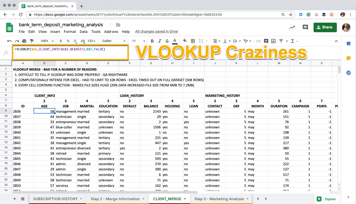
VLOOKUP that Takes Forever to Compute
…And here are the 3 lines of code that do the VLOOKUP join in R.
# 3 Lines of Code - Accomplishes VLOOKUP saving us hours!
data_joined_tbl <- sheets[4:7] %>%
    map(~ read_excel(path = path_to_excel_file, sheet = .)) %>%
    reduce(left_join)
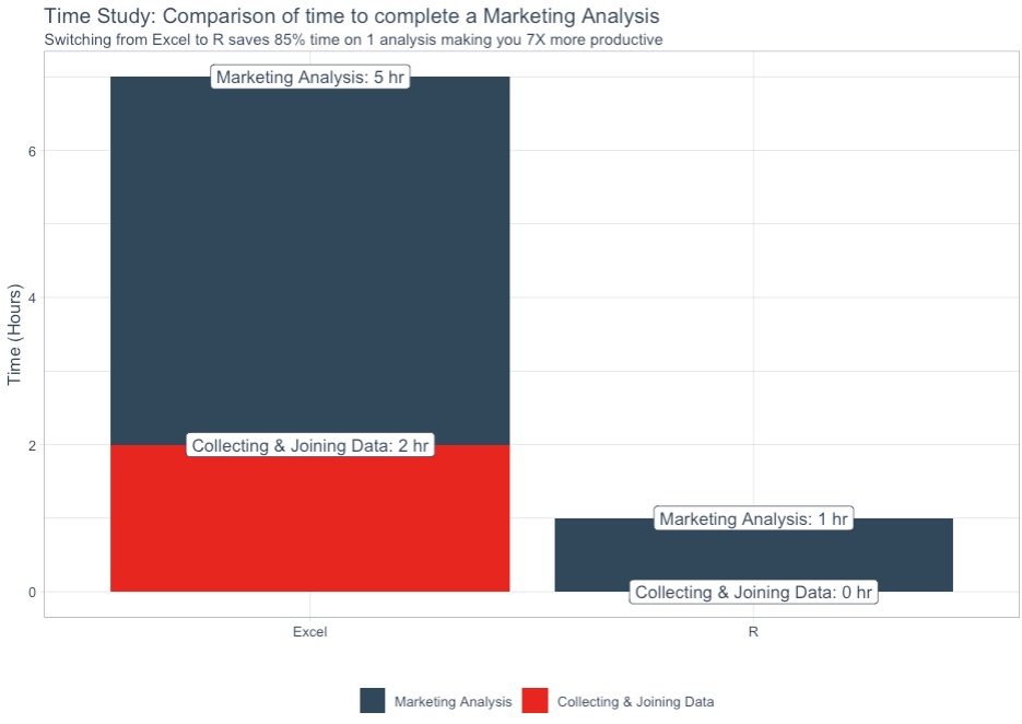
Time Study - Save 6 hours (minimum)
We’ll also uncover a shocking Time Study were we estimate switching from Excel to R saving 6 hours on the marketing analysis, making you a minimum of 7X more productive in the process. Once you develop the code (see how in Part 2 of the series), you can rinse-and-repeat boosting your productivity to 10X and beyond!
The VLOOKUP can be performed in R with 3 lines of code
Video Tutorial - Marketing Case Study
The Excel to R - 3-part Series - is also available as a video tutorial from our recent Learning Lab - Excel to R - Marketing Case Study. If you prefer video walkthroughs, then check this video out. If you want to attend the next Learning Lab live or get copies of the recordings, sign up for Learning Labs here.
Learning Lab - Excel to R - Marketing Case Study
Contents
Marketing Case Study - Term Deposit Analysis
This 3-Part series follows a real-world study that companies like Bank of America an others that provide Certificates of Deposit (CDs) (Term Deposits) would go through to analyze customer purchasing behavior.

The bank is interested in contacting customers that are likely to enroll in a Term Deposit (CD for a fixed term). The banks love these products because they can earn interest on the customers money. More enrollments means more revenue for the bank.
Requirements
Here’s what you’ll need to follow along:
-
Excel or Google Sheets to view the Excel File
-
Install R and RStudio. Install the following libraries with the install.packages() function: tidyverse, readxl, recipes, tidyquant, and ggrepel. These will be used throughout the 3-part series.
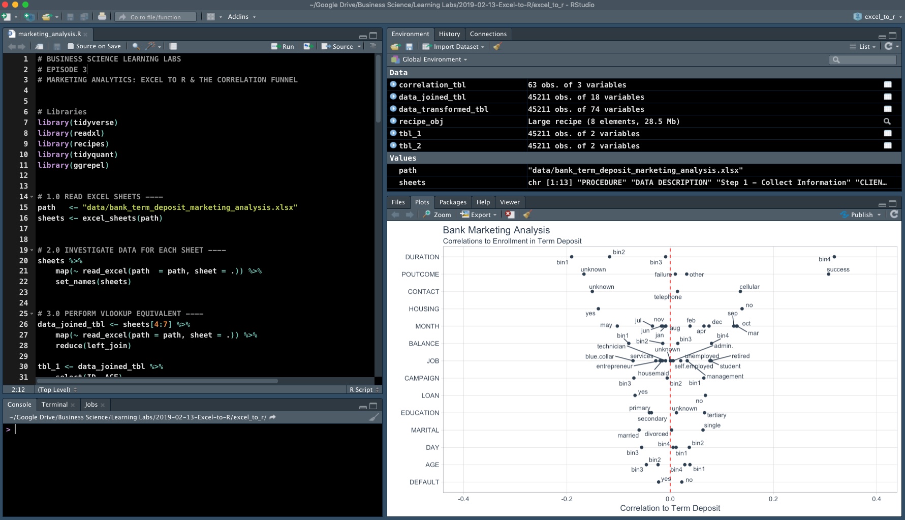
RStudio Desktop IDE
Get the Data
The dataset we’ll use is a modified version of the “Bank Marketing Data Set” provided by the UCI Machine Learning Repository. The version we will use is in an Excel file with multiple tabs covering the business process.
In the data folder, download the Excel File, “bank_term_deposit_marketing_analysis.xlsx”.
Business Process
The Excel File is setup like many business processes where there are multiple tabs indicating steps in the business process.
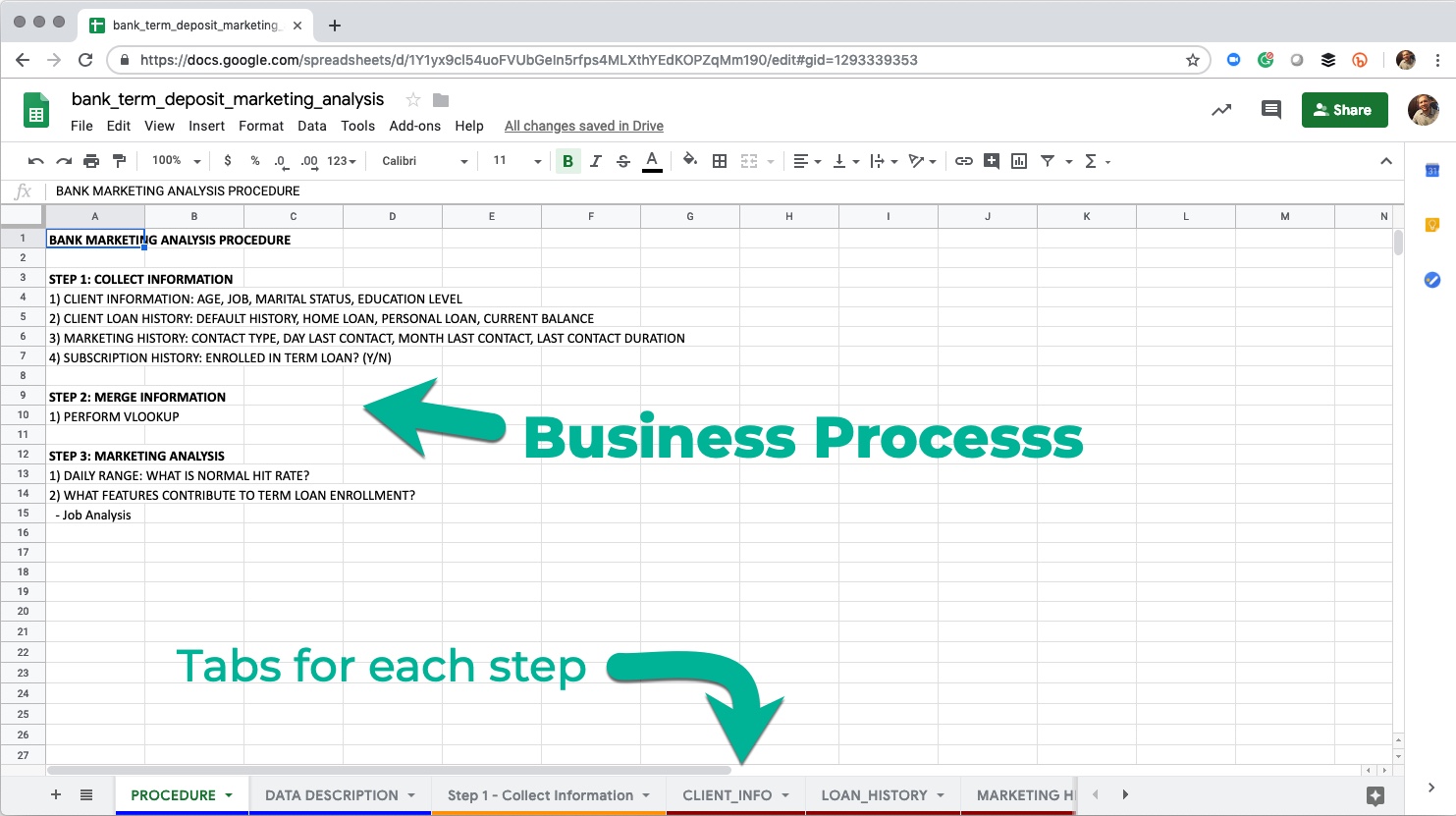
Excel File Contents
The Business Process has 3 Steps:
-
Collect Data - The goal is to collect data that can be mined for relationships to Term Deposit enrollment. This is where Client Information, Loan History, Marketing History, and Term Loan (Product Enrollment) Information is pulled into Excel.
-
Merge Information - This is where the VLOOKUP is performed to join the 4 spreadsheet tables from the first step.
-
Perform Marketing Analysis - This is where the business analyst performs the Marketing Study mining the data for relationships between to the customer enrollments in the term deposit product.
Implementing the Process in Excel and R
Let’s investigate the first 2 steps of the process to show what’s going on and what happens inside of Excel when doing a VLOOKUP.
Step 1 - Collect Information
This step is already done, which is basically taking tables from a SQL database and pulling the information into Excel in the four worksheets:
- CLIENT_INFO
- LOAN_HISTORY
- MARKETING HISTORY
- SUBSCRIPTION HISTORY
1. Client Information
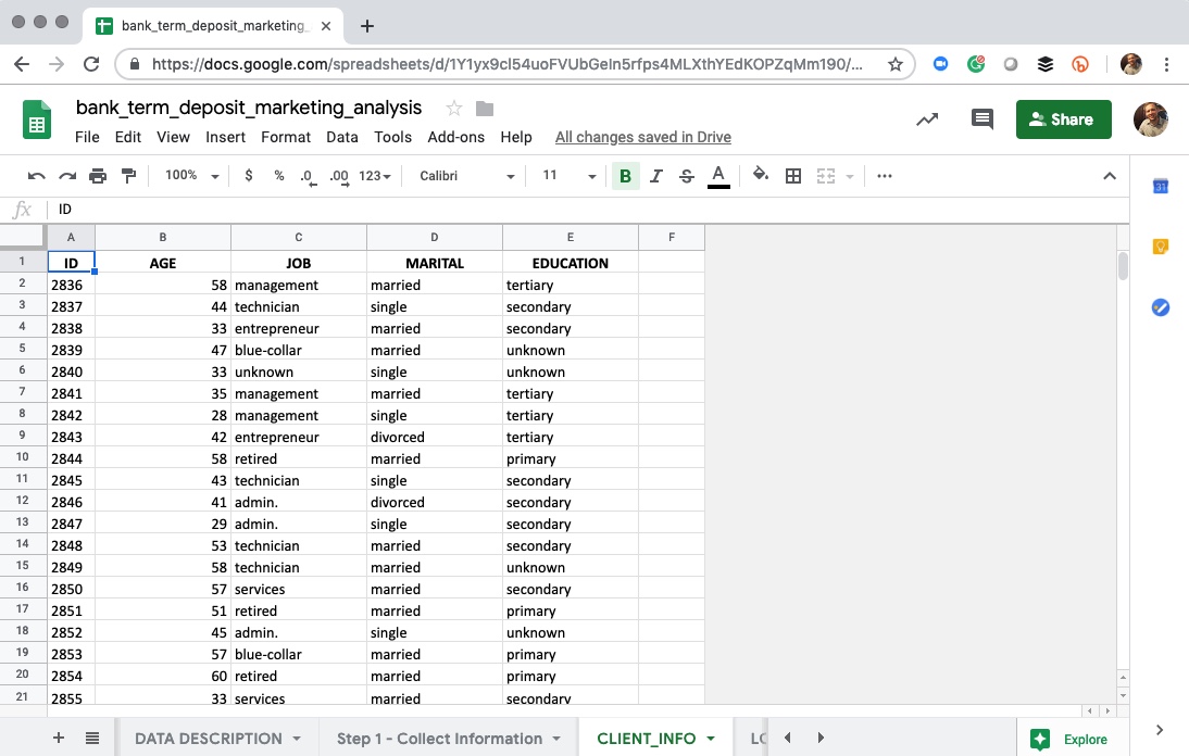
Client Information
This worksheet includes the following features:
- ID - Unique Client ID
- AGE - Age of the client
- JOB - Current job category
- MARITAL - Marital status (single, married, divorced)
- EDUCATION - Education level (primary, secondary, tertiary, unknown)
2. Loan History
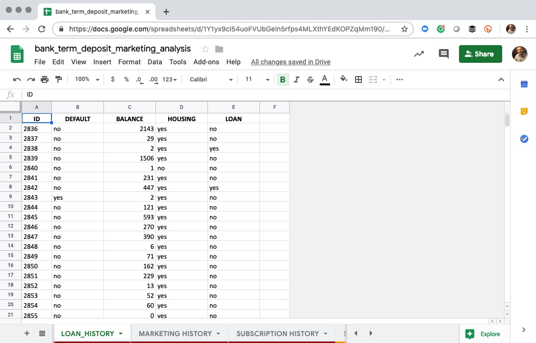
Loan History
This worksheet includes the following features:
- ID - Unique Client ID
- DEFAULT - Has credit in default (yes/no)
- BALANCE - Average yearly balance
- HOUSING - Home loan (yes/no)
- LOAN - Personal loan (yes/no)
3. Marketing History
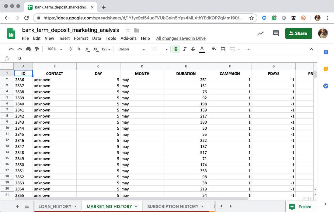
Marketing History
This worksheet includes the following features:
- ID - Unique Client ID
- CONTACT - The type of contact (cellular, telephone, unknown)
- DAY - Day of the month when the client was last contacted
- MONTH - Month of the year when the client was last contacted
- DURATION - Duration of the last contact in seconds
- CAMPAIGN - Number of contacts performed during this campaign
- PDAYS - Number of days passed after the client was last contacted
- PREVIOUS - Number of contacts performed before this campaign
- POUTCOME - Outcome of the previous marketing campaign (success, failure, other, unknown)
4. Subscription History
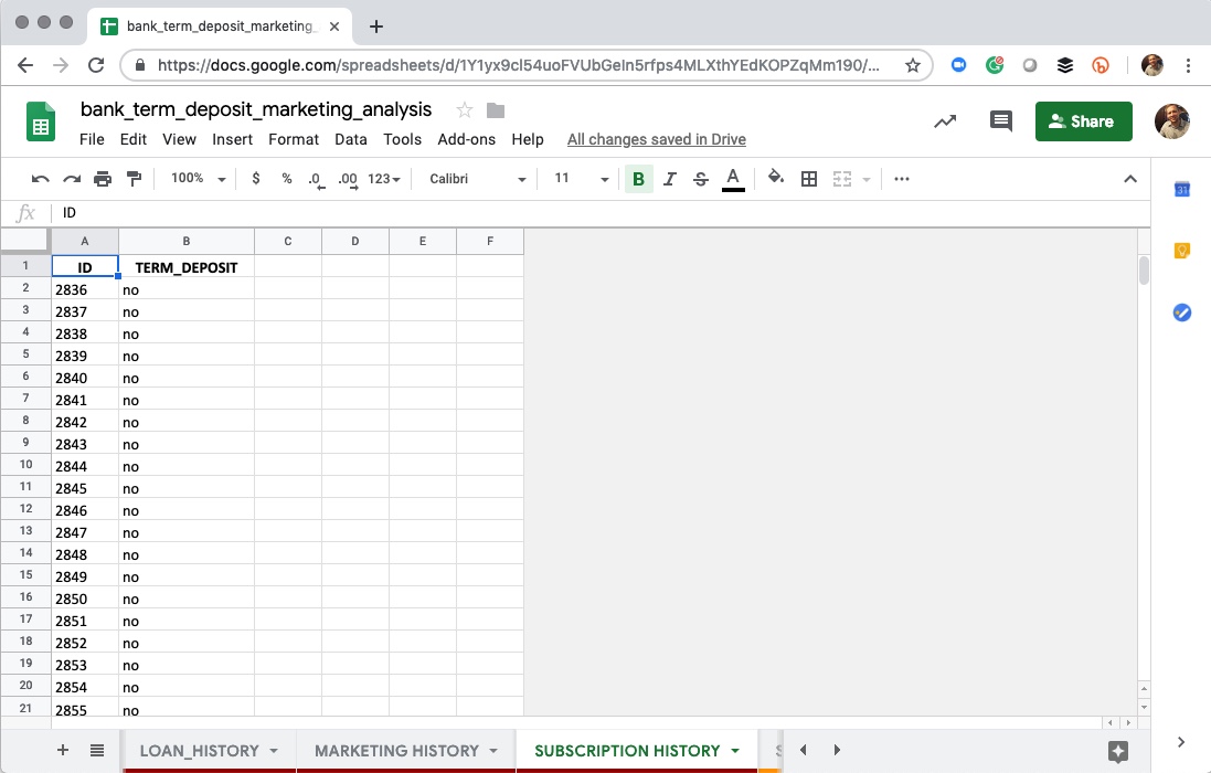
Subscription History
This worksheet includes the following features:
- ID - Unique Client ID
- TERM_DEPOSIT - Whether or not the customer enrolled in the program (yes/no)
Step 2 - Merge the Data
Excel: Joining Data
This is very challenging in Excel because of several reasons I will get to in a minute. First, we want to get each of the 4 worksheets (CLIENT_INFO, LOAN_HISTORY, MARKETING HISTORY, and SUBSCRIPTION HISTORY) into one combined table where all of the data is joined using the “ID” field. Here’s how we attempt to do the VLOOKUP on our 45,000 row data set.
VLOOKUP Attempt
This is a VLOOKUP that I attempted. It combines data from 4 worksheets - the end data set was supposed to be 45,211 rows by 18 columns. After letting the Excel Application spin for about 20 minutes I decided to truncate the rows to 10,000 or about 20% of the data. The VLOOKUP then worked.

VLOOKUP that Grinds My Mac to a Halt
VLOOKUP Process
The general process is as follows:
- We create column indexes for each of the columns we want to pull in (row 7). these correspond the column positions in each of the 4 worksheets of “feeder data” (data feeding the
VLOOKUP)
- We build the first
VLOOKUP() in cell B9
- 1st argument: We key in on the ID field (column A) making sure to remember the dollar sign (
$A9) in front of A to lock into the “A” column
- 2nd Argument: We select the data for the first worksheet (
CLIENT_INFO) remembering to lock in the entire data with $ signs in front of the first column and row and the last column and row ($A$2:$E$45212)
- 3rd Argument: We then add the column index in row 7 making sure to lock the row in with a dollar sign (
B$7)
- 4th Argument: We add
FALSE to ensure exact matching (we don’t want partial matches… do we ever???).
- We drag the VLOOKUP across and down to fill in the first 4 columns (AGE to EDUCATION)
- We then repeat this process for the remaining 3 worksheets
Excel: The Pain
This was painful for 3 Reasons:
-
Errors: I made at least 3 mistakes when performing the VLOOKUP. At various points, I forgot dollar signs before dragging, and the output looked very similar to what I was going for. It took me a lot of unnecessary time to debug. Plus - If I had someone checking my work, I doubt that they would have caught all of the errors. This is a QA nightmare!
-
Computational Intensity: We are not dealing with a lot of data. 45K rows by 18 columns is normal. Yet, by the 4th VLOOKUP, Excel had my computer spinning in an “I’m thinking and this is going to take a really long time” way. I eventually trimmed the data set to the first 10K rows (20% of data) and it worked, but that’s terrible because I need to evaluate all of the data.
-
My Excel File Doubled, I only replicated 20% of data: Excel is not efficient. Each VLOOKUP is stored as a function in every cell (45K x 18 = 810K functions), which causes file sizes to increase exponentially. My file’s size went from 4MB to 7.2MB during the VLOOKUP - and I only performed the VLOOKUP on 10K rows (20% of the data).
R: Joining Data
Joining Multiple Excel Sheets in R
Here’s how simple the process is in R. First, I load the tidyverse and readxl.
-
tidyverse: A meta-package that contains several workhorse packages including dplyr, ggplot2, and purrr.
-
readxl: A light-weight package for reading Excel files.
# Load Libraries
library(tidyverse)
library(readxl)
Next, we setup a string which is the path to our file. My file is located in a folder named data that is in my home directory. Use getwd() to identify your home directory.
# Setup path
path_to_excel_file <- "data/bank_term_deposit_marketing_analysis.xlsx"
Next, let’s determine what sheets exist in the Excel file. We can use excel_sheets() to determine this.
# Read excel sheets
sheets <- excel_sheets(path_to_excel_file)
sheets
##  [1] "PROCEDURE"                    "DATA DESCRIPTION"
##  [3] "Step 1 - Collect Information" "CLIENT_INFO"
##  [5] "LOAN_HISTORY"                 "MARKETING HISTORY"
##  [7] "SUBSCRIPTION HISTORY"         "Step 2 - Merge Information"
##  [9] "CLIENT_MERGE"                 "Step 3 - Marketing Analysis"
## [11] "DAILY RANGE"                  "JOB ANALYSIS"
## [13] "Sheet3"
We want to read in the data from sheet 4 (“CLIENT_INFO”) through sheet 7 (“SUBSCRIPTION HISTORY”). Here’s how we can do it in one pipe.
# 3 Lines of Code - Accomplishes VLOOKUP saving us hours!
data_joined_tbl <- sheets[4:7] %>%
    map(~ read_excel(path = path_to_excel_file, sheet = .)) %>%
    reduce(left_join, by = "ID")
For those that want to understand what the code above is doing:
Just to prove that each worksheet was joined appropriately, the next line of code shows the first 10 rows of the resulting 45,211 row x 18 column tibble.
data_joined_tbl %>%
    slice(1:10) %>%
    knitr::kable()
| ID |
AGE |
JOB |
MARITAL |
EDUCATION |
DEFAULT |
BALANCE |
HOUSING |
LOAN |
CONTACT |
DAY |
MONTH |
DURATION |
CAMPAIGN |
PDAYS |
PREVIOUS |
POUTCOME |
TERM_DEPOSIT |
| 2836 |
58 |
management |
married |
tertiary |
no |
2143 |
yes |
no |
unknown |
5 |
may |
261 |
1 |
-1 |
0 |
unknown |
no |
| 2837 |
44 |
technician |
single |
secondary |
no |
29 |
yes |
no |
unknown |
5 |
may |
151 |
1 |
-1 |
0 |
unknown |
no |
| 2838 |
33 |
entrepreneur |
married |
secondary |
no |
2 |
yes |
yes |
unknown |
5 |
may |
76 |
1 |
-1 |
0 |
unknown |
no |
| 2839 |
47 |
blue-collar |
married |
unknown |
no |
1506 |
yes |
no |
unknown |
5 |
may |
92 |
1 |
-1 |
0 |
unknown |
no |
| 2840 |
33 |
unknown |
single |
unknown |
no |
1 |
no |
no |
unknown |
5 |
may |
198 |
1 |
-1 |
0 |
unknown |
no |
| 2841 |
35 |
management |
married |
tertiary |
no |
231 |
yes |
no |
unknown |
5 |
may |
139 |
1 |
-1 |
0 |
unknown |
no |
| 2842 |
28 |
management |
single |
tertiary |
no |
447 |
yes |
yes |
unknown |
5 |
may |
217 |
1 |
-1 |
0 |
unknown |
no |
| 2843 |
42 |
entrepreneur |
divorced |
tertiary |
yes |
2 |
yes |
no |
unknown |
5 |
may |
380 |
1 |
-1 |
0 |
unknown |
no |
| 2844 |
58 |
retired |
married |
primary |
no |
121 |
yes |
no |
unknown |
5 |
may |
50 |
1 |
-1 |
0 |
unknown |
no |
| 2845 |
43 |
technician |
single |
secondary |
no |
593 |
yes |
no |
unknown |
5 |
may |
55 |
1 |
-1 |
0 |
unknown |
no |
R: The Gain
R just saved us about 2 hours of work. In 3 lines of code, we read the each of the 4 excel sheets and iteratively joined using an exact match on the “ID” column for all 45,211 customers.
# 3 Lines of Code - Accomplishes VLOOKUP saving us hours!
data_joined_tbl <- sheets[4:7] %>%
    map(~ read_excel(path = path_to_excel_file, sheet = .)) %>%
    reduce(left_join)
The best part - You don’t need to even know what this code does. Just make sure the “ID” column is the only matching column in each of the worksheets that you want to join. Copy-and-paste it the next time you are in a similar situation.
Step 3 - Marketing Analysis
Excel: Pivot Tables and Pivot Charts Galore
The approach we normally take in Excel is investigating features one-by-one with Pivot Tables and Pivot Charts. This is a great way to interactively explore the data, but it’s also time consuming. Let’s follow the analytical process for a few iterations.
Daily Hit Rate - Baseline
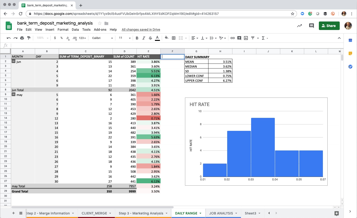
We want to assess the hit rate (how many clients enroll vs total clients) to get a baseline for our analysis. One way we can do so is by analyzing the daily activity. We spend 30 minutes or so coming up with a nice sheet that looks something like this. We can see pretty clearly that our daily range is around 3.5% with a range of about 1% to 6% on most given days.
Daily Hit Rate
With a baseline hit rate in hand, we can then start to assess which features yield a higher hit rate.
Job Analysis
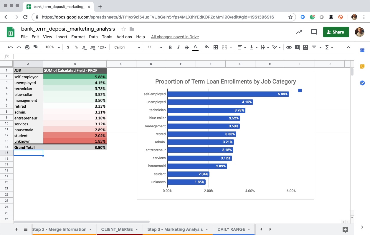
We spend another 15 minutes or so on our next analysis, which is gauging which job categories yield higher hit rates than the baseline 3.5%.
Job Analysis
From this, we develop a story that “self-employed” customers are almost double the hit-rate and therefore are better to contact. What we don’t realize is that we are only considering 20% of the data, which is heavily biased because it’s only the two months of a much longer time series data set.
Excel: The Pain
We’ve just spent 3 hours collecting data, combining data, and analyzing 2 features, and we are no closer to the truth because we only have 20% of the data set in our VLOOKUP. We have an estimated 4 more hours of work (16 more features x 15 minutes/feature of analysis) to get through the whole data set. The entire estimated analysis is going to take 7+ hours and this doesn’t include writing a report.
At 7+ hours for analysis not including writing a report, it’s going to be a long day unless we use a better tool for the job.
R: Correlation Funnel
Rather than go through all 18 features one-by-one, we can let the insights come to us by way of a special technique called a Correlation Funnel.
Correlation Funnel
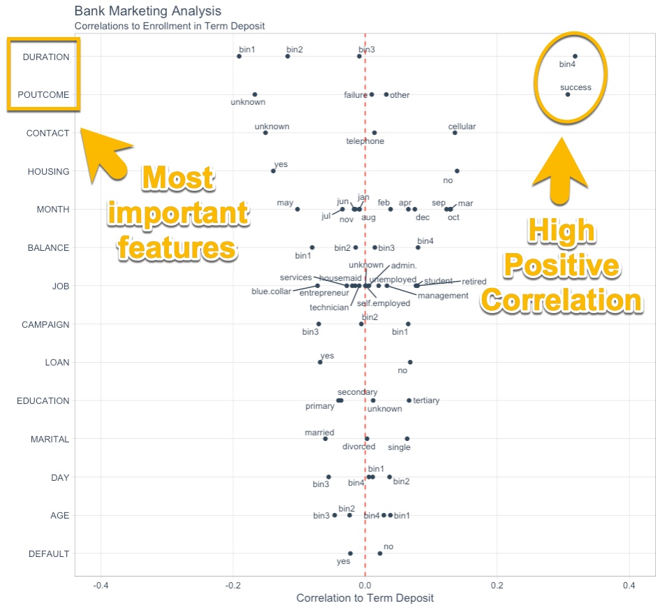
Here’s what the Correlation Funnel looks like on this data set. In the next post, we’ll show you how to set it up.
R: The Gain
More Accurate Results:
The top features are Duration of call (“DURATION”) and Previous Outcome (“POUTCOME”). Having POUTCOME = “SUCCESS” or DURATION >= 319 results in a high likelihood of enrolling in Term Deposit.
It turns out that JOB = “self.employed” (identified in the Excel Job Analysis) has very little correlation to Term Deposit as shown in the Correlation Funnel. This is the issue with only using 20% of a data set for a cross section of time. Making sacrifices to accommodate the VLOOKUP caused us to incorrectly identify self employed customers rather than focus on the most important features including Previous Outcome and Call Duration.
Time Savings:
The correlation funnel takes minutes to set up, and we can generate valuable insights quickly. At 1 hour for setup (first time), the estimate time savings is 6 hours or about 85% more efficient versus Excel (7+ hours).
Better yet, I can repeatedly use the script in Part 2 so future Matt will get a time savings of approaching the full 7 hours.
Summary of Time Savings
Just for kicks, I’ll show a quick visual using ggplot2 of the time savings from switching from Excel to R for 1 Marketing Analysis (excluding Reporting, which saves even more time).
First, convert the time savings estimate to a tibble in an appropriate format for ggplot2.
# Summarize Time Savings
time_savings_tbl <- tibble(
    type  = c("Collecting & Joining Data", "Marketing Analysis"),
    R     = c(0, 1),
    Excel = c(2, 5)
) %>%
    mutate(type = type %>% factor(levels=c("Marketing Analysis", "Collecting & Joining Data"))) %>%
    gather(key = "tool", value = "time", -type, factor_key = F)

time_savings_tbl
## # A tibble: 4 x 3
##   type                      tool   time
##   <fct>                     <chr> <dbl>
## 1 Collecting & Joining Data R         0
## 2 Marketing Analysis        R         1
## 3 Collecting & Joining Data Excel     2
## 4 Marketing Analysis        Excel     5
Plot the result using ggplot2 package. I use the tidyquant theme, which makes business-ready plots.
time_savings_tbl %>%
    ggplot(aes(x = tool, y = time, fill = type)) +
    geom_col() +
    geom_label(aes(label = str_glue("{type}: {time} hr")),
               position= "stack",
               fill = "white", color = "#2c3e50"
               ) +
    tidyquant::scale_fill_tq() +
    tidyquant::theme_tq() +
    labs(
        title = "Time Study: Comparison of time to complete a Marketing Analysis",
        subtitle = "Switching from Excel to R saves 85% time on 1 analysis making you 7X more productive",
        y = "Time (Hours)", x = "", fill = ""
    )
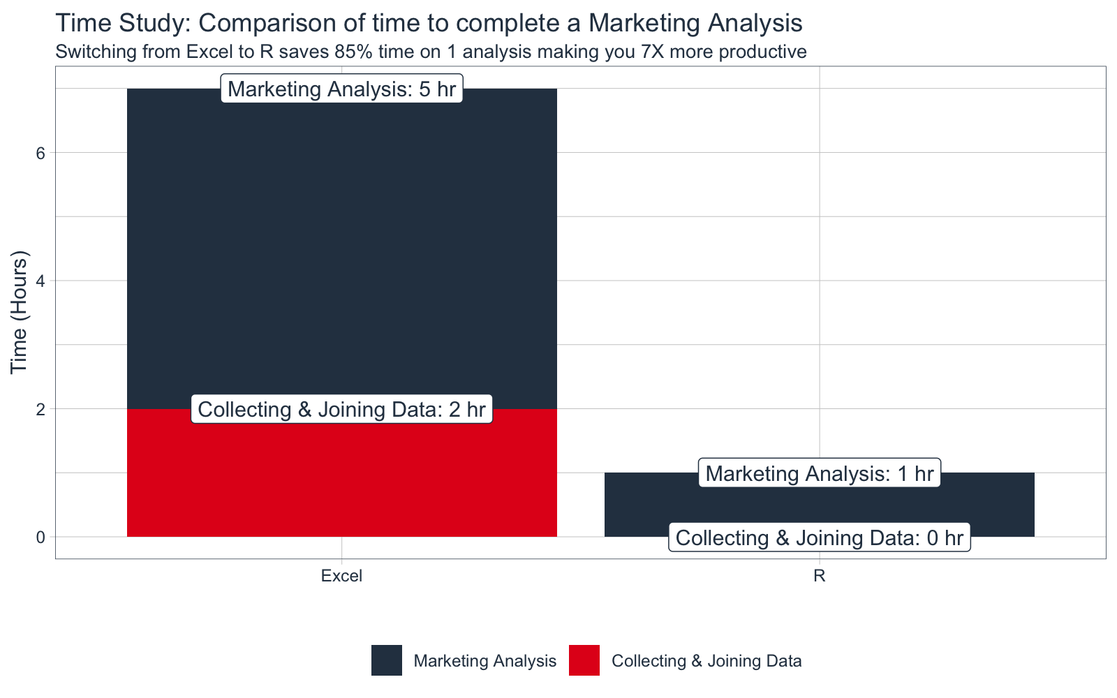
The Time Study visualization makes is pretty clear that switching from Excel to R is much more efficient. In the next article we’ll see how the Marketing Analysis can be performed in R using the Correlation Funnel.
Conclusion
In the first part of the Marketing Case Study, we’ve seen how Excel has glaring issues with:
VLOOKUP Breaks Down - Does not handle medium-size data well, easy for errors to go unnoticed- Inefficient Analysis - 7+ hours to perform the marketing evaluation
- Inaccurate Analysis - Because of the data limitation (we were only able to use 20%), the Job Analysis was inaccurate
We’ve also seen that R has benefits in joining data (saving about 2-3 hours per complex VLOOKUP), reducing errors in the process, and making QA’s job easier (someone has to review).
The real benefits will become much clearer once we get to the Correlation Funnel. This drops the analysis time dramatically for a total time savings of about 90% - 100% (R at 0-1 hours as compared to Excel as 7+ hours)
We’ll cover the Correlation Funnel in the next article, “Excel to R for Marketing, Part 2 - The Correlation Funnel” (Coming Soon).
Learning R is not that difficult:
Finally, if you want to learn R, be sure to check out our Business Science University Curriculum below. We have an integrated 3-Course R-Track that will teach you everything you need to be effective as a data scientist. And, you can do it - going from no prior knowledge to advanced in weeks.
References