Time Series Machine Learning (and Feature Engineering) in R
Written by Matt Dancho
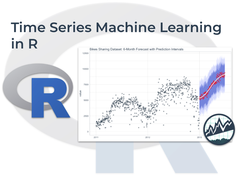
Machine learning is a powerful way to analyze Time Series. With innovations in the tidyverse modeling infrastructure (tidymodels), we now have a common set of packages to perform machine learning in R. These packages include parsnip, recipes, tune, and workflows. But what about Machine Learning with Time Series Data? The key is Feature Engineering. (Read the updated article at Business Science)
The timetk package has a feature engineering innovation in version 0.1.3. A recipe step called step_timeseries_signature() for Time Series Feature Engineering that is designed to fit right into the tidymodels workflow for machine learning with timeseries data.
The small innovation creates 25+ time series features, which has a big impact in improving our machine learning models. Further, these “core features” are the basis for creating 200+ time-series features to improve forecasting performance. Let’s see how to do Time Series Machine Learning in R.
Time Series Feature Engineering
with the Time Series Signature

Use feature engineering with timetk to forecast
The time series signature is a collection of useful engineered features that describe the time series index of a time-based data set. It contains a 25+ time-series features that can be used to forecast time series that contain common seasonal and trend patterns:
-
✅ Trend in Seconds Granularity: index.num
-
✅ Yearly Seasonality: Year, Month, Quarter
-
✅ Weekly Seasonality: Week of Month, Day of Month, Day of Week, and more
-
✅ Daily Seasonality: Hour, Minute, Second
-
✅ Weekly Cyclic Patterns: 2 weeks, 3 weeks, 4 weeks
We can then build 200+ of new features from these core 25+ features by applying well-thought-out time series feature engineering strategies.
Time Series Forecast Strategy
6-Month Forecast of Bike Transaction Counts
In this tutorial, the user will learn methods to implement machine learning to predict future outcomes in a time-based data set. The tutorial example uses a well known time series dataset, the Bike Sharing Dataset, from the UCI Machine Learning Repository. The objective is to build a model and predict the next 6-months of Bike Sharing daily transaction counts.
Feature Engineering Strategy
I’ll use timetk to build a basic Machine Learning Feature Set using the new step_timeseries_signature() function that is part of preprocessing specification via the recipes package. I’ll show how you can add interaction terms, dummy variables, and more to build 200+ new features from the pre-packaged feature set.
Machine Learning Strategy
We’ll then perform Time Series Machine Learning using parsnip and workflows to construct and train a GLM-based time series machine learning model. The model is evaluated on out-of-sample data. A final model is trained on the full dataset, and extended to a future dataset containing 6-months to daily timestamp data.

Time Series Forecast using Feature Engineering
How to Learn Forecasting Beyond this Tutorial
I can’t possibly show you all the Time Series Forecasting techniques you need to learn in this post, which is why I have a NEW Advanced Time Series Forecasting Course on its way. The course includes detailed explanations from 3 Time Series Competitions. We go over competition solutions and show how you can integrate the key strategies into your organization’s time series forecasting projects. Check out the course page, and Sign-Up to get notifications on the Advanced Time Series Forecasting Course (Coming soon).
Need to improve forecasting at your company?
I have the Advanced Time Series Forecasting Course (Coming Soon). This course pulls forecasting strategies from experts that have placed 1st and 2nd solutions in 3 of the most important Time Series Competitions. Learn the strategies that win forecasting competitions. Then apply them to your time series projects.
Join the waitlist to get notified of the Course Launch!
Join the Advanced Time Series Course Waitlist
Prerequisites
Please use timetk 0.1.3 or greater for this tutorial. You can install via remotes::install_github("business-science/timetk") until released on CRAN.
Before we get started, load the following packages.
library(workflows)
library(parsnip)
library(recipes)
library(yardstick)
library(glmnet)
library(tidyverse)
library(tidyquant)
library(timetk) # Use >= 0.1.3, remotes::install_github("business-science/timetk")
Data
We’ll be using the Bike Sharing Dataset from the UCI Machine Learning Repository. Download the data and select the “day.csv” file which is aggregated to daily periodicity.
# Read data
bikes <- read_csv("2020-03-18-timeseries-ml/day.csv")

# Select date and count
bikes_tbl <- bikes %>%
    select(dteday, cnt) %>%
    rename(date  = dteday,
           value = cnt)
A visualization will help understand how we plan to tackle the problem of forecasting the data. We’ll split the data into two regions: a training region and a testing region.
# Visualize data and training/testing regions
bikes_tbl %>%
    ggplot(aes(x = date, y = value)) +
    geom_rect(xmin = as.numeric(ymd("2012-07-01")),
              xmax = as.numeric(ymd("2013-01-01")),
              ymin = 0, ymax = 10000,
              fill = palette_light()[[4]], alpha = 0.01) +
    annotate("text", x = ymd("2011-10-01"), y = 7800,
             color = palette_light()[[1]], label = "Train Region") +
    annotate("text", x = ymd("2012-10-01"), y = 1550,
             color = palette_light()[[1]], label = "Test Region") +
    geom_point(alpha = 0.5, color = palette_light()[[1]]) +
    labs(title = "Bikes Sharing Dataset: Daily Scale", x = "") +
    theme_tq()
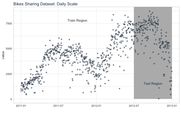
Split the data into train and test sets at “2012-07-01”.
# Split into training and test sets
train_tbl <- bikes_tbl %>% filter(date < ymd("2012-07-01"))
test_tbl  <- bikes_tbl %>% filter(date >= ymd("2012-07-01"))
Modeling
Start with the training set, which has the “date” and “value” columns.
# Training set
train_tbl
## # A tibble: 547 x 2
##    date       value
##    <date>     <dbl>
##  1 2011-01-01   985
##  2 2011-01-02   801
##  3 2011-01-03  1349
##  4 2011-01-04  1562
##  5 2011-01-05  1600
##  6 2011-01-06  1606
##  7 2011-01-07  1510
##  8 2011-01-08   959
##  9 2011-01-09   822
## 10 2011-01-10  1321
## # … with 537 more rows
Recipe Preprocessing Specification
The first step is to add the time series signature to the training set, which will be used this to learn the patterns. New in timetk 0.1.3 is integration with the recipes R package:
-
The recipes package allows us to add preprocessing steps that are applied sequentially as part of a data transformation pipeline.
-
The timetk has step_timeseries_signature(), which is used to add a number of features that can help machine learning models.
# Add time series signature
recipe_spec_timeseries <- recipe(value ~ ., data = train_tbl) %>%
    step_timeseries_signature(date)
When we apply the prepared recipe prep() using the bake() function, we go from 2 features to 29 features! Yes, 25+ new columns were added from the timestamp “date” feature. These are features we can use in our machine learning models and build on top of. .
bake(prep(recipe_spec_timeseries), new_data = train_tbl)
## # A tibble: 547 x 29
##    date       value date_index.num date_year date_year.iso date_half
##    <date>     <dbl>          <int>     <int>         <int>     <int>
##  1 2011-01-01   985     1293840000      2011          2010         1
##  2 2011-01-02   801     1293926400      2011          2010         1
##  3 2011-01-03  1349     1294012800      2011          2011         1
##  4 2011-01-04  1562     1294099200      2011          2011         1
##  5 2011-01-05  1600     1294185600      2011          2011         1
##  6 2011-01-06  1606     1294272000      2011          2011         1
##  7 2011-01-07  1510     1294358400      2011          2011         1
##  8 2011-01-08   959     1294444800      2011          2011         1
##  9 2011-01-09   822     1294531200      2011          2011         1
## 10 2011-01-10  1321     1294617600      2011          2011         1
## # … with 537 more rows, and 23 more variables: date_quarter <int>,
## #   date_month <int>, date_month.xts <int>, date_month.lbl <ord>,
## #   date_day <int>, date_hour <int>, date_minute <int>, date_second <int>,
## #   date_hour12 <int>, date_am.pm <int>, date_wday <int>, date_wday.xts <int>,
## #   date_wday.lbl <ord>, date_mday <int>, date_qday <int>, date_yday <int>,
## #   date_mweek <int>, date_week <int>, date_week.iso <int>, date_week2 <int>,
## #   date_week3 <int>, date_week4 <int>, date_mday7 <int>
Building Engineered Features on Top of our Recipe
Next is where the magic happens. I apply various preprocessing steps to improve the modeling behavior to go from 29 features to 225 engineered features! If you wish to learn more, I have an Advanced Time Series course that will help you learn these techniques.
recipe_spec_final <- recipe_spec_timeseries %>%
    step_rm(date) %>%
    step_rm(contains("iso"),
            contains("second"), contains("minute"), contains("hour"),
            contains("am.pm"), contains("xts")) %>%
    step_normalize(contains("index.num"), date_year) %>%
    step_interact(~ date_month.lbl * date_day) %>%
    step_interact(~ date_month.lbl * date_mweek) %>%
    step_interact(~ date_month.lbl * date_wday.lbl * date_yday) %>%
    step_dummy(contains("lbl"), one_hot = TRUE)

bake(prep(recipe_spec_final), new_data = train_tbl)
## # A tibble: 547 x 225
##    value date_index.num date_year date_half date_quarter date_month date_day
##    <dbl>          <dbl>     <dbl>     <int>        <int>      <int>    <int>
##  1   985          -1.73    -0.705         1            1          1        1
##  2   801          -1.72    -0.705         1            1          1        2
##  3  1349          -1.71    -0.705         1            1          1        3
##  4  1562          -1.71    -0.705         1            1          1        4
##  5  1600          -1.70    -0.705         1            1          1        5
##  6  1606          -1.70    -0.705         1            1          1        6
##  7  1510          -1.69    -0.705         1            1          1        7
##  8   959          -1.68    -0.705         1            1          1        8
##  9   822          -1.68    -0.705         1            1          1        9
## 10  1321          -1.67    -0.705         1            1          1       10
## # … with 537 more rows, and 218 more variables: date_wday <int>,
## #   date_mday <int>, date_qday <int>, date_yday <int>, date_mweek <int>,
## #   date_week <int>, date_week2 <int>, date_week3 <int>, date_week4 <int>,
## #   date_mday7 <int>, date_month.lbl.L_x_date_day <dbl>,
## #   date_month.lbl.Q_x_date_day <dbl>, date_month.lbl.C_x_date_day <dbl>,
## #   `date_month.lbl^4_x_date_day` <dbl>, `date_month.lbl^5_x_date_day` <dbl>,
## #   `date_month.lbl^6_x_date_day` <dbl>, `date_month.lbl^7_x_date_day` <dbl>,
## #   `date_month.lbl^8_x_date_day` <dbl>, `date_month.lbl^9_x_date_day` <dbl>,
## #   `date_month.lbl^10_x_date_day` <dbl>, `date_month.lbl^11_x_date_day` <dbl>,
## #   date_month.lbl.L_x_date_mweek <dbl>, date_month.lbl.Q_x_date_mweek <dbl>,
## #   date_month.lbl.C_x_date_mweek <dbl>, `date_month.lbl^4_x_date_mweek` <dbl>,
## #   `date_month.lbl^5_x_date_mweek` <dbl>,
## #   `date_month.lbl^6_x_date_mweek` <dbl>,
## #   `date_month.lbl^7_x_date_mweek` <dbl>,
## #   `date_month.lbl^8_x_date_mweek` <dbl>,
## #   `date_month.lbl^9_x_date_mweek` <dbl>,
## #   `date_month.lbl^10_x_date_mweek` <dbl>,
## #   `date_month.lbl^11_x_date_mweek` <dbl>,
## #   date_month.lbl.L_x_date_wday.lbl.L <dbl>,
## #   date_month.lbl.Q_x_date_wday.lbl.L <dbl>,
## #   date_month.lbl.C_x_date_wday.lbl.L <dbl>,
## #   `date_month.lbl^4_x_date_wday.lbl.L` <dbl>,
## #   `date_month.lbl^5_x_date_wday.lbl.L` <dbl>,
## #   `date_month.lbl^6_x_date_wday.lbl.L` <dbl>,
## #   `date_month.lbl^7_x_date_wday.lbl.L` <dbl>,
## #   `date_month.lbl^8_x_date_wday.lbl.L` <dbl>,
## #   `date_month.lbl^9_x_date_wday.lbl.L` <dbl>,
## #   `date_month.lbl^10_x_date_wday.lbl.L` <dbl>,
## #   `date_month.lbl^11_x_date_wday.lbl.L` <dbl>,
## #   date_month.lbl.L_x_date_wday.lbl.Q <dbl>,
## #   date_month.lbl.Q_x_date_wday.lbl.Q <dbl>,
## #   date_month.lbl.C_x_date_wday.lbl.Q <dbl>,
## #   `date_month.lbl^4_x_date_wday.lbl.Q` <dbl>,
## #   `date_month.lbl^5_x_date_wday.lbl.Q` <dbl>,
## #   `date_month.lbl^6_x_date_wday.lbl.Q` <dbl>,
## #   `date_month.lbl^7_x_date_wday.lbl.Q` <dbl>,
## #   `date_month.lbl^8_x_date_wday.lbl.Q` <dbl>,
## #   `date_month.lbl^9_x_date_wday.lbl.Q` <dbl>,
## #   `date_month.lbl^10_x_date_wday.lbl.Q` <dbl>,
## #   `date_month.lbl^11_x_date_wday.lbl.Q` <dbl>,
## #   date_month.lbl.L_x_date_wday.lbl.C <dbl>,
## #   date_month.lbl.Q_x_date_wday.lbl.C <dbl>,
## #   date_month.lbl.C_x_date_wday.lbl.C <dbl>,
## #   `date_month.lbl^4_x_date_wday.lbl.C` <dbl>,
## #   `date_month.lbl^5_x_date_wday.lbl.C` <dbl>,
## #   `date_month.lbl^6_x_date_wday.lbl.C` <dbl>,
## #   `date_month.lbl^7_x_date_wday.lbl.C` <dbl>,
## #   `date_month.lbl^8_x_date_wday.lbl.C` <dbl>,
## #   `date_month.lbl^9_x_date_wday.lbl.C` <dbl>,
## #   `date_month.lbl^10_x_date_wday.lbl.C` <dbl>,
## #   `date_month.lbl^11_x_date_wday.lbl.C` <dbl>,
## #   `date_month.lbl.L_x_date_wday.lbl^4` <dbl>,
## #   `date_month.lbl.Q_x_date_wday.lbl^4` <dbl>,
## #   `date_month.lbl.C_x_date_wday.lbl^4` <dbl>,
## #   `date_month.lbl^4_x_date_wday.lbl^4` <dbl>,
## #   `date_month.lbl^5_x_date_wday.lbl^4` <dbl>,
## #   `date_month.lbl^6_x_date_wday.lbl^4` <dbl>,
## #   `date_month.lbl^7_x_date_wday.lbl^4` <dbl>,
## #   `date_month.lbl^8_x_date_wday.lbl^4` <dbl>,
## #   `date_month.lbl^9_x_date_wday.lbl^4` <dbl>,
## #   `date_month.lbl^10_x_date_wday.lbl^4` <dbl>,
## #   `date_month.lbl^11_x_date_wday.lbl^4` <dbl>,
## #   `date_month.lbl.L_x_date_wday.lbl^5` <dbl>,
## #   `date_month.lbl.Q_x_date_wday.lbl^5` <dbl>,
## #   `date_month.lbl.C_x_date_wday.lbl^5` <dbl>,
## #   `date_month.lbl^4_x_date_wday.lbl^5` <dbl>,
## #   `date_month.lbl^5_x_date_wday.lbl^5` <dbl>,
## #   `date_month.lbl^6_x_date_wday.lbl^5` <dbl>,
## #   `date_month.lbl^7_x_date_wday.lbl^5` <dbl>,
## #   `date_month.lbl^8_x_date_wday.lbl^5` <dbl>,
## #   `date_month.lbl^9_x_date_wday.lbl^5` <dbl>,
## #   `date_month.lbl^10_x_date_wday.lbl^5` <dbl>,
## #   `date_month.lbl^11_x_date_wday.lbl^5` <dbl>,
## #   `date_month.lbl.L_x_date_wday.lbl^6` <dbl>,
## #   `date_month.lbl.Q_x_date_wday.lbl^6` <dbl>,
## #   `date_month.lbl.C_x_date_wday.lbl^6` <dbl>,
## #   `date_month.lbl^4_x_date_wday.lbl^6` <dbl>,
## #   `date_month.lbl^5_x_date_wday.lbl^6` <dbl>,
## #   `date_month.lbl^6_x_date_wday.lbl^6` <dbl>,
## #   `date_month.lbl^7_x_date_wday.lbl^6` <dbl>,
## #   `date_month.lbl^8_x_date_wday.lbl^6` <dbl>,
## #   `date_month.lbl^9_x_date_wday.lbl^6` <dbl>,
## #   `date_month.lbl^10_x_date_wday.lbl^6` <dbl>,
## #   `date_month.lbl^11_x_date_wday.lbl^6` <dbl>,
## #   date_month.lbl.L_x_date_yday <dbl>, date_month.lbl.Q_x_date_yday <dbl>, …
Model Specification
Next, let’s create a model specification. We’ll use a glmnet.
model_spec_glmnet <- linear_reg(mode = "regression", penalty = 10, mixture = 0.7) %>%
    set_engine("glmnet")
Workflow
We can mary up the preprocessing recipe and the model using a workflow().
workflow_glmnet <- workflow() %>%
    add_recipe(recipe_spec_final) %>%
    add_model(model_spec_glmnet)

workflow_glmnet
## ══ Workflow ════════════════════════════════════════════════════════════════════════════════════════════════════════════════════
## Preprocessor: Recipe
## Model: linear_reg()
##
## ── Preprocessor ────────────────────────────────────────────────────────────────────────────────────────────────────────────────
## 8 Recipe Steps
##
## ● step_timeseries_signature()
## ● step_rm()
## ● step_rm()
## ● step_normalize()
## ● step_interact()
## ● step_interact()
## ● step_interact()
## ● step_dummy()
##
## ── Model ───────────────────────────────────────────────────────────────────────────────────────────────────────────────────────
## Linear Regression Model Specification (regression)
##
## Main Arguments:
##   penalty = 10
##   mixture = 0.7
##
## Computational engine: glmnet
Training
The workflow can be trained with the fit() function.
workflow_trained <- workflow_glmnet %>% fit(data = train_tbl)
Visualize the Test (Validation) Forecast
With a suitable model in hand, we can forecast using the “test” set for validation purposes.
prediction_tbl <- workflow_trained %>%
    predict(test_tbl) %>%
    bind_cols(test_tbl)

prediction_tbl
## # A tibble: 184 x 3
##    .pred date       value
##    <dbl> <date>     <dbl>
##  1 6903. 2012-07-01  5531
##  2 7030. 2012-07-02  6227
##  3 6960. 2012-07-03  6660
##  4 6931. 2012-07-04  7403
##  5 6916. 2012-07-05  6241
##  6 6934. 2012-07-06  6207
##  7 7169. 2012-07-07  4840
##  8 6791. 2012-07-08  4672
##  9 6837. 2012-07-09  6569
## 10 6766. 2012-07-10  6290
## # … with 174 more rows
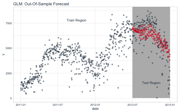
Visualize the results using ggplot().
ggplot(aes(x = date), data = bikes_tbl) +
    geom_rect(xmin = as.numeric(ymd("2012-07-01")),
              xmax = as.numeric(ymd("2013-01-01")),
              ymin = 0, ymax = 10000,
              fill = palette_light()[[4]], alpha = 0.01) +
    annotate("text", x = ymd("2011-10-01"), y = 7800,
             color = palette_light()[[1]], label = "Train Region") +
    annotate("text", x = ymd("2012-10-01"), y = 1550,
             color = palette_light()[[1]], label = "Test Region") +
    geom_point(aes(x = date, y = value),
               alpha = 0.5, color = palette_light()[[1]]) +
    # Add predictions
    geom_point(aes(x = date, y = .pred), data = prediction_tbl,
               alpha = 0.5, color = palette_light()[[2]]) +
    theme_tq() +
    labs(title = "GLM: Out-Of-Sample Forecast")
Validation Accuracy (Out of Sample)
The Out-of-Sample Forecast Accuracy can be measured with yardstick.
# Calculating forecast error
prediction_tbl %>% metrics(value, .pred)
## # A tibble: 3 x 3
##   .metric .estimator .estimate
##   <chr>   <chr>          <dbl>
## 1 rmse    standard    1377.
## 2 rsq     standard       0.422
## 3 mae     standard    1022.
Next we can visualize the residuals of the test set. The residuals of the model aren’t perfect, but we can work with it. The residuals show that the model predicts low in October and high in December.
prediction_tbl %>%
    ggplot(aes(x = date, y = value - .pred)) +
    geom_hline(yintercept = 0, color = "black") +
    geom_point(color = palette_light()[[1]], alpha = 0.5) +
    geom_smooth(span = 0.05, color = "red") +
    geom_smooth(span = 1.00, se = FALSE) +
    theme_tq() +
    labs(title = "GLM Model Residuals, Out-of-Sample", x = "") +
    scale_y_continuous(limits = c(-5000, 5000))
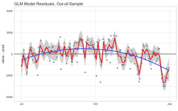
At this point you might go back to the model and try tweaking features using interactions or polynomial terms, adding other features that may be known in the future (e.g. temperature of day can be forecasted relatively accurately within 7 days), or try a completely different modeling technique with the hope of better predictions on the test set. Once you feel that your model is optimized, move on the final step of forecasting.
This accuracy can be improved significantly with Competition-Level Forecasting Strategies. And, guess what?! I teach these strategies in my NEW Advanced Time Series Forecasting Course (coming soon). Register for the waitlist to get notified. 👇
Learn algorithms that win competitions
I have the Advanced Time Series Forecasting Course (Coming Soon). This course pulls forecasting strategies from experts that have placed 1st and 2nd solutions in 3 of the most important Time Series Competitions. Learn the strategies that win forecasting competitions. Then apply them to your time series projects.
Join the waitlist to get notified of the Course Launch!
Forecasting Future Data
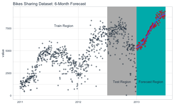
Let’s use our model to predict What are the expected future values for the next six months. The first step is to create the date sequence. Let’s use tk_get_timeseries_summary() to review the summary of the dates from the original dataset, “bikes”.
# Extract bikes index
idx <- bikes_tbl %>% tk_index()

# Get time series summary from index
bikes_summary <- idx %>% tk_get_timeseries_summary()
The first six parameters are general summary information.
bikes_summary[1:6]
## # A tibble: 1 x 6
##   n.obs start      end        units scale tzone
##   <int> <date>     <date>     <chr> <chr> <chr>
## 1   731 2011-01-01 2012-12-31 days  day   UTC
The second six parameters are the periodicity information.
bikes_summary[7:12]
## # A tibble: 1 x 6
##   diff.minimum diff.q1 diff.median diff.mean diff.q3 diff.maximum
##          <dbl>   <dbl>       <dbl>     <dbl>   <dbl>        <dbl>
## 1        86400   86400       86400     86400   86400        86400
From the summary, we know that the data is 100% regular because the median and mean differences are 86400 seconds or 1 day. We don’t need to do any special inspections when we use tk_make_future_timeseries(). If the data was irregular, meaning weekends or holidays were excluded, you’d want to account for this. Otherwise your forecast would be inaccurate.
idx_future <- idx %>% tk_make_future_timeseries(n_future = 180)

future_tbl <- tibble(date = idx_future)

future_tbl
## # A tibble: 180 x 1
##    date
##    <date>
##  1 2013-01-01
##  2 2013-01-02
##  3 2013-01-03
##  4 2013-01-04
##  5 2013-01-05
##  6 2013-01-06
##  7 2013-01-07
##  8 2013-01-08
##  9 2013-01-09
## 10 2013-01-10
## # … with 170 more rows
Retrain the model specification on the full data set, then predict the next 6-months.
future_predictions_tbl <- workflow_glmnet %>%
    fit(data = bikes_tbl) %>%
    predict(future_tbl) %>%
    bind_cols(future_tbl)
Visualize the forecast.
bikes_tbl %>%
    ggplot(aes(x = date, y = value)) +
    geom_rect(xmin = as.numeric(ymd("2012-07-01")),
              xmax = as.numeric(ymd("2013-01-01")),
              ymin = 0, ymax = 10000,
              fill = palette_light()[[4]], alpha = 0.01) +
    geom_rect(xmin = as.numeric(ymd("2013-01-01")),
              xmax = as.numeric(ymd("2013-07-01")),
              ymin = 0, ymax = 10000,
              fill = palette_light()[[3]], alpha = 0.01) +
    annotate("text", x = ymd("2011-10-01"), y = 7800,
             color = palette_light()[[1]], label = "Train Region") +
    annotate("text", x = ymd("2012-10-01"), y = 1550,
             color = palette_light()[[1]], label = "Test Region") +
    annotate("text", x = ymd("2013-4-01"), y = 1550,
             color = palette_light()[[1]], label = "Forecast Region") +
    geom_point(alpha = 0.5, color = palette_light()[[1]]) +
    # future data
    geom_point(aes(x = date, y = .pred), data = future_predictions_tbl,
               alpha = 0.5, color = palette_light()[[2]]) +
    geom_smooth(aes(x = date, y = .pred), data = future_predictions_tbl,
                method = 'loess') +
    labs(title = "Bikes Sharing Dataset: 6-Month Forecast", x = "") +
    theme_tq()
Forecast Error
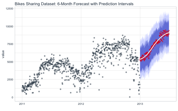
A forecast is never perfect. We need prediction intervals to account for the variance from the model predictions to the actual data. There’s a number of methods to achieve this. We’ll follow the prediction interval methodology from Forecasting: Principles and Practice.
# Calculate standard deviation of residuals
test_resid_sd <- prediction_tbl %>%
    summarize(stdev = sd(value - .pred))

future_predictions_tbl <- future_predictions_tbl %>%
    mutate(
        lo.95 = .pred - 1.96 * test_resid_sd$stdev,
        lo.80 = .pred - 1.28 * test_resid_sd$stdev,
        hi.80 = .pred + 1.28 * test_resid_sd$stdev,
        hi.95 = .pred + 1.96 * test_resid_sd$stdev
    )
Now, plotting the forecast with the prediction intervals.
bikes_tbl %>%
    ggplot(aes(x = date, y = value)) +
    geom_point(alpha = 0.5, color = palette_light()[[1]]) +
    geom_ribbon(aes(y = .pred, ymin = lo.95, ymax = hi.95),
                data = future_predictions_tbl,
                fill = "#D5DBFF", color = NA, size = 0) +
    geom_ribbon(aes(y = .pred, ymin = lo.80, ymax = hi.80, fill = key),
                data = future_predictions_tbl,
                fill = "#596DD5", color = NA, size = 0, alpha = 0.8) +
    geom_point(aes(x = date, y = .pred), data = future_predictions_tbl,
               alpha = 0.5, color = palette_light()[[2]]) +
    geom_smooth(aes(x = date, y = .pred), data = future_predictions_tbl,
                method = 'loess', color = "white") +
    labs(title = "Bikes Sharing Dataset: 6-Month Forecast with Prediction Intervals", x = "") +
    theme_tq()
My Key Points on Time Series Machine Learning
Forecasting using the time series signature can be very accurate especially when time-based patterns are present in the underlying data. As with most machine learning applications, the prediction is only as good as the patterns in the data. Forecasting using this approach may not be suitable when patterns are not present or when the future is highly uncertain (i.e. past is not a suitable predictor of future performance). However, in may situations the time series signature can provide an accurate forecast.
External Regressors - A huge benefit: One benefit to the machine learning approach that was not covered in this tutorial is that _correlated features (including non-time-based) can be included in the analysis. This is called adding External Regressors - examples include adding data from weather, financial, energy, google analytics, email providers, and more. For example, one can expect that experts in Bike Sharing analytics have access to historical temperature and weather patterns, wind speeds, and so on that could have a significant affect on bicycle sharing. The beauty of this method is these features can easily be incorporated into the model and prediction.
There is a whole lot more to time series forecasting that we did not cover (read on). 👇
How to Learn Time Series Forecasting?
Here are some techniques you need to learn to become good at forecasting. These techiques are absolutely critical to developing forecasts that will return ROI to your company:
- ✅ Preprocessing
- ✅ Feature engineering using Lagged Features and External Regressors
- ✅ Hyperparameter Tuning
- ✅ Time series cross validation
- ✅ Using Multiple Modeling Techniques
- ✅ Leveraging Autocorrelation
- ✅ and more.
All of these techiniques are covered in my upcoming Advanced Time Series Course (Register Here). I teach Competition-Winning Forecast Strategies too:
- ✅ Ensembling Strategies and Techniques
- ✅ Deep Learning Algorithms leveraging Recurrent Neural Networks
- ✅ Feature-Based Model Selection
And a whole lot more! It should be simple by now - Join my course waitlist.
Join the Advanced Time Series Course Waitlist