Demo Week: Time Series Machine Learning with timetk
Written by Matt Dancho

We’re into the second day of Business Science Demo Week. What’s demo week? Every day this week we are demoing an R package: tidyquant (Monday), timetk (Tuesday), sweep (Wednesday), tibbletime (Thursday) and h2o (Friday)! That’s five packages in five days! We’ll give you intel on what you need to know about these packages to go from zero to hero. Second up is timetk, your toolkit for time series in R. Here we go!
Demo Week Demos:
Get The Best Resources In Data Science. Every Friday!
Sign up for our free "5 Topic Friday" Newsletter. Every week, I'll send you the five coolest topics in data science for business that I've found that week. These could be new R packages, free books, or just some fun to end the week on.
Sign Up For Five-Topic-Friday!
timetk: What’s It Used For?
There are three main uses:
-
Time series machine learning: Using regression algorithms to forecast
-
Making future time series indicies: Extract, explore, and extend a time series index using patterns in the time-base
-
Coercing (converting) between time classes (e.g. between tbl, xts, zoo, ts): Consistent coercion makes working in the various time classes much easier!
We’ll go over time series ML and coercion today. The second (extracting and making future time series) will be touched on in time series ML as this is very critical to prediction accuracy.
Load Libraries
We’ll need two libraries today:
tidyquant: For getting data and loading the tidyverse behind the scenestimetk: Toolkit for working with time series in R
If you haven’t done so already, install the packages:
# Install packages
install.packages("timetk")
install.packages("tidyquant")
Load the libraries.
# Load libraries
library(timetk)     # Toolkit for working with time series in R
library(tidyquant)  # Loads tidyverse, financial pkgs, used to get data
Data
We’ll get data using the tq_get() function from tidyquant. The data comes from FRED: Beer, Wine, and Distilled Alcoholic Beverages Sales.
# Beer, Wine, Distilled Alcoholic Beverages, in Millions USD
beer_sales_tbl <- tq_get("S4248SM144NCEN", get = "economic.data", from = "2010-01-01", to = "2016-12-31")

beer_sales_tbl
## # A tibble: 84 x 2
##          date price
##        <date> <int>
##  1 2010-01-01  6558
##  2 2010-02-01  7481
##  3 2010-03-01  9475
##  4 2010-04-01  9424
##  5 2010-05-01  9351
##  6 2010-06-01 10552
##  7 2010-07-01  9077
##  8 2010-08-01  9273
##  9 2010-09-01  9420
## 10 2010-10-01  9413
## # ... with 74 more rows
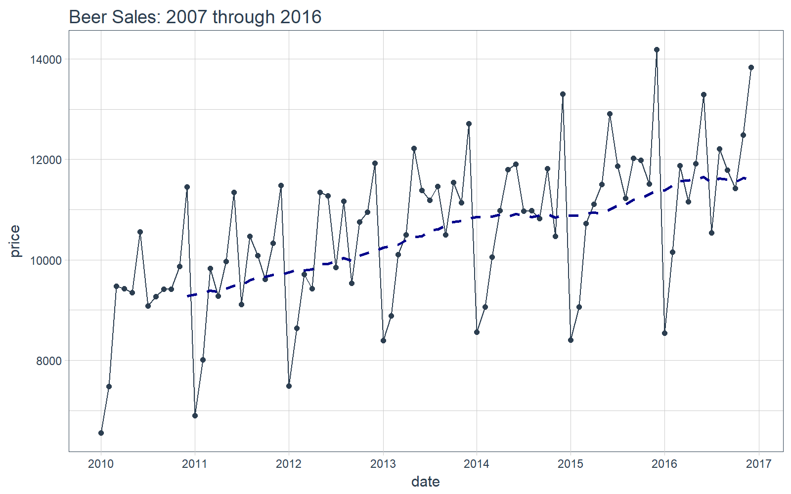
It’s a good idea to visualize the data so we know what we’re working with. Visualization is particularly important for time series analysis and forecasting (as we see during time series machine learning). We’ll use tidyquant charting tools: mainly geom_ma(ma_fun = SMA, n = 12) to add a 12-period simple moving average to get an idea of the trend. We can also see there appears to be both trend (moving average is increasing in a relatively linear pattern) and some seasonality (peaks and troughs tend to occur at specific months).
# Plot Beer Sales
beer_sales_tbl %>%
    ggplot(aes(date, price)) +
    geom_line(col = palette_light()[1]) +
    geom_point(col = palette_light()[1]) +
    geom_ma(ma_fun = SMA, n = 12, size = 1) +
    theme_tq() +
    scale_x_date(date_breaks = "1 year", date_labels = "%Y") +
    labs(title = "Beer Sales: 2007 through 2016")
Now that you have a feel for the time series we’ll be working with today, let’s move onto the demo!
DEMO: timetk
We’ve split this demo into two parts. First, we’ll follow a workflow for time series machine learning. Second, we’ll check out coercion tools.
Part 1: Time Series Machine Learning
Time series machine learning is a great way to forecast time series data, but before we get started here are a couple pointers for this demo:
-
Key Insight: The time series signature ~ timestamp information expanded column-wise into a feature set ~ is used to perform machine learning.
-
Objective: We’ll predict the next 12 months of data for the time series using the time series signature.
We’ll go through a workflow that can be used to perform time series machine learning. You’ll see how several timetk functions can help with this process. We’ll do machine learning with a simple lm() linear regression, and you will see how powerful and accurate this can be when a time series signature is used. Further, you should think about what other more powerful machine learning algorithms can be used such as xgboost, glmnet (LASSO), and others.
Step 0: Review data
Just to show our starting point, let’s print out our beer_sales_tbl.
# Starting point
beer_sales_tbl
## # A tibble: 84 x 2
##          date price
##        <date> <int>
##  1 2010-01-01  6558
##  2 2010-02-01  7481
##  3 2010-03-01  9475
##  4 2010-04-01  9424
##  5 2010-05-01  9351
##  6 2010-06-01 10552
##  7 2010-07-01  9077
##  8 2010-08-01  9273
##  9 2010-09-01  9420
## 10 2010-10-01  9413
## # ... with 74 more rows
We can quickly get a feel for the time series using tk_index() to extract the index and tk_get_timeseries_summary() to retrieve summary information of the index. We use glimpse() to output in a nice format for review.
beer_sales_tbl %>%
    tk_index() %>%
    tk_get_timeseries_summary() %>%
    glimpse()
## Observations: 1
## Variables: 12
## $ n.obs        <int> 84
## $ start        <date> 2010-01-01
## $ end          <date> 2016-12-01
## $ units        <chr> "days"
## $ scale        <chr> "month"
## $ tzone        <chr> "UTC"
## $ diff.minimum <dbl> 2419200
## $ diff.q1      <dbl> 2592000
## $ diff.median  <dbl> 2678400
## $ diff.mean    <dbl> 2629475
## $ diff.q3      <dbl> 2678400
## $ diff.maximum <dbl> 2678400
We can see important features like start, end, units, etc. We also have the quantiles of the time-diffs (difference in seconds between observations), which is useful for assessing the degree of regularity. Because the scale is monthly, the number of seconds between each month follows an irregular distribution.
Step 1: Augment Time Series Signature
The tk_augment_timeseries_signature() function expands out the timestamp information column-wise into a machine learning feature set, adding columns of time series information to the original data frame.
# Augment (adds data frame columns)
beer_sales_tbl_aug <- beer_sales_tbl %>%
    tk_augment_timeseries_signature()

beer_sales_tbl_aug
## # A tibble: 84 x 30
##          date price  index.num    diff  year year.iso  half quarter
##        <date> <int>      <int>   <int> <int>    <int> <int>   <int>
##  1 2010-01-01  6558 1262304000      NA  2010     2009     1       1
##  2 2010-02-01  7481 1264982400 2678400  2010     2010     1       1
##  3 2010-03-01  9475 1267401600 2419200  2010     2010     1       1
##  4 2010-04-01  9424 1270080000 2678400  2010     2010     1       2
##  5 2010-05-01  9351 1272672000 2592000  2010     2010     1       2
##  6 2010-06-01 10552 1275350400 2678400  2010     2010     1       2
##  7 2010-07-01  9077 1277942400 2592000  2010     2010     2       3
##  8 2010-08-01  9273 1280620800 2678400  2010     2010     2       3
##  9 2010-09-01  9420 1283299200 2678400  2010     2010     2       3
## 10 2010-10-01  9413 1285891200 2592000  2010     2010     2       4
## # ... with 74 more rows, and 22 more variables: month <int>,
## #   month.xts <int>, month.lbl <ord>, day <int>, hour <int>,
## #   minute <int>, second <int>, hour12 <int>, am.pm <int>,
## #   wday <int>, wday.xts <int>, wday.lbl <ord>, mday <int>,
## #   qday <int>, yday <int>, mweek <int>, week <int>, week.iso <int>,
## #   week2 <int>, week3 <int>, week4 <int>, mday7 <int>
Step 2: Model
Apply any regression model to the data. We’ll use lm(). Note that we drop the date and diff columns. Most algorithms do not work with dates, and the diff column is not useful for machine learning (it’s more useful for finding time gaps in the data).
# linear regression model used, but can use any model
fit_lm <- lm(price ~ ., data = select(beer_sales_tbl_aug, -c(date, diff)))

summary(fit_lm)
##
## Call:
## lm(formula = price ~ ., data = select(beer_sales_tbl_aug, -c(date,
##     diff)))
##
## Residuals:
##    Min     1Q Median     3Q    Max
## -447.3 -145.4  -18.2  169.8  421.4
##
## Coefficients: (16 not defined because of singularities)
##                Estimate Std. Error t value Pr(>|t|)
## (Intercept)   3.660e+08  1.245e+08   2.940 0.004738 **
## index.num     5.900e-03  2.003e-03   2.946 0.004661 **
## year         -1.974e+05  6.221e+04  -3.173 0.002434 **
## year.iso      1.159e+04  6.546e+03   1.770 0.082006 .
## half         -2.132e+03  6.107e+02  -3.491 0.000935 ***
## quarter      -1.239e+04  2.190e+04  -0.566 0.573919
## month        -3.910e+03  7.355e+03  -0.532 0.597058
## month.xts            NA         NA      NA       NA
## month.lbl.L          NA         NA      NA       NA
## month.lbl.Q  -1.643e+03  2.069e+02  -7.942 8.59e-11 ***
## month.lbl.C   8.368e+02  5.139e+02   1.628 0.108949
## month.lbl^4   6.452e+02  1.344e+02   4.801 1.18e-05 ***
## month.lbl^5   7.563e+02  4.241e+02   1.783 0.079852 .
## month.lbl^6   3.206e+02  1.609e+02   1.992 0.051135 .
## month.lbl^7  -3.537e+02  1.867e+02  -1.894 0.063263 .
## month.lbl^8   3.687e+02  3.217e+02   1.146 0.256510
## month.lbl^9          NA         NA      NA       NA
## month.lbl^10  6.339e+02  2.240e+02   2.830 0.006414 **
## month.lbl^11         NA         NA      NA       NA
## day                  NA         NA      NA       NA
## hour                 NA         NA      NA       NA
## minute               NA         NA      NA       NA
## second               NA         NA      NA       NA
## hour12               NA         NA      NA       NA
## am.pm                NA         NA      NA       NA
## wday         -8.264e+01  1.898e+01  -4.353 5.63e-05 ***
## wday.xts             NA         NA      NA       NA
## wday.lbl.L           NA         NA      NA       NA
## wday.lbl.Q   -7.109e+02  1.093e+02  -6.503 2.13e-08 ***
## wday.lbl.C    2.355e+02  1.336e+02   1.763 0.083273 .
## wday.lbl^4    8.033e+01  1.133e+02   0.709 0.481281
## wday.lbl^5    6.480e+01  8.029e+01   0.807 0.422951
## wday.lbl^6    2.276e+01  8.200e+01   0.278 0.782319
## mday                 NA         NA      NA       NA
## qday         -1.362e+02  2.418e+02  -0.563 0.575326
## yday         -2.356e+02  1.416e+02  -1.664 0.101627
## mweek        -1.670e+02  1.477e+02  -1.131 0.262923
## week         -1.764e+02  1.890e+02  -0.933 0.354618
## week.iso      2.315e+02  1.256e+02   1.842 0.070613 .
## week2        -1.235e+02  1.547e+02  -0.798 0.428283
## week3                NA         NA      NA       NA
## week4                NA         NA      NA       NA
## mday7                NA         NA      NA       NA
## ---
## Signif. codes:  0 '***' 0.001 '**' 0.01 '*' 0.05 '.' 0.1 ' ' 1
##
## Residual standard error: 260.4 on 57 degrees of freedom
## Multiple R-squared:  0.9798,	Adjusted R-squared:  0.9706
## F-statistic: 106.4 on 26 and 57 DF,  p-value: < 2.2e-16
Step 3: Build Future (New) Data
Use tk_index() to extract the index.
# Retrieves the timestamp information
beer_sales_idx <- beer_sales_tbl %>%
    tk_index()

tail(beer_sales_idx)
## [1] "2016-07-01" "2016-08-01" "2016-09-01" "2016-10-01" "2016-11-01"
## [6] "2016-12-01"
Make a future index from the existing index with tk_make_future_timeseries. The function internally checks the periodicity and returns the correct sequence. Note that we have a whole vignette on how to make future time series, which is helpful due to the complexity of the topic.
# Make future index
future_idx <- beer_sales_idx %>%
    tk_make_future_timeseries(n_future = 12)

future_idx
##  [1] "2017-01-01" "2017-02-01" "2017-03-01" "2017-04-01" "2017-05-01"
##  [6] "2017-06-01" "2017-07-01" "2017-08-01" "2017-09-01" "2017-10-01"
## [11] "2017-11-01" "2017-12-01"
From the future index, use tk_get_timeseries_signature() to turn index into time signature data frame.
new_data_tbl <- future_idx %>%
    tk_get_timeseries_signature()

new_data_tbl
## # A tibble: 12 x 29
##         index  index.num    diff  year year.iso  half quarter month
##        <date>      <int>   <int> <int>    <int> <int>   <int> <int>
##  1 2017-01-01 1483228800      NA  2017     2016     1       1     1
##  2 2017-02-01 1485907200 2678400  2017     2017     1       1     2
##  3 2017-03-01 1488326400 2419200  2017     2017     1       1     3
##  4 2017-04-01 1491004800 2678400  2017     2017     1       2     4
##  5 2017-05-01 1493596800 2592000  2017     2017     1       2     5
##  6 2017-06-01 1496275200 2678400  2017     2017     1       2     6
##  7 2017-07-01 1498867200 2592000  2017     2017     2       3     7
##  8 2017-08-01 1501545600 2678400  2017     2017     2       3     8
##  9 2017-09-01 1504224000 2678400  2017     2017     2       3     9
## 10 2017-10-01 1506816000 2592000  2017     2017     2       4    10
## 11 2017-11-01 1509494400 2678400  2017     2017     2       4    11
## 12 2017-12-01 1512086400 2592000  2017     2017     2       4    12
## # ... with 21 more variables: month.xts <int>, month.lbl <ord>,
## #   day <int>, hour <int>, minute <int>, second <int>, hour12 <int>,
## #   am.pm <int>, wday <int>, wday.xts <int>, wday.lbl <ord>,
## #   mday <int>, qday <int>, yday <int>, mweek <int>, week <int>,
## #   week.iso <int>, week2 <int>, week3 <int>, week4 <int>,
## #   mday7 <int>
Step 4: Predict the New Data
Use the predict() function for your regression model. Note that we drop the index and diff columns, the same as before when using the lm() function.
# Make predictions
pred <- predict(fit_lm, newdata = select(new_data_tbl, -c(index, diff)))

predictions_tbl <- tibble(
    date  = future_idx,
    value = pred
    )

predictions_tbl
## # A tibble: 12 x 2
##          date     value
##        <date>     <dbl>
##  1 2017-01-01  9509.122
##  2 2017-02-01 10909.189
##  3 2017-03-01 12281.835
##  4 2017-04-01 11378.678
##  5 2017-05-01 13080.710
##  6 2017-06-01 13583.471
##  7 2017-07-01 11529.085
##  8 2017-08-01 12984.939
##  9 2017-09-01 11859.998
## 10 2017-10-01 12331.419
## 11 2017-11-01 13047.033
## 12 2017-12-01 13940.003
Step 5: Compare Actual vs Predictions
We can use tq_get() to retrieve the actual data. Note that we don’t have all of the data for comparison, but we can at least compare the first several months of actual values.
actuals_tbl <- tq_get("S4248SM144NCEN", get = "economic.data", from = "2017-01-01", to = "2017-12-31")
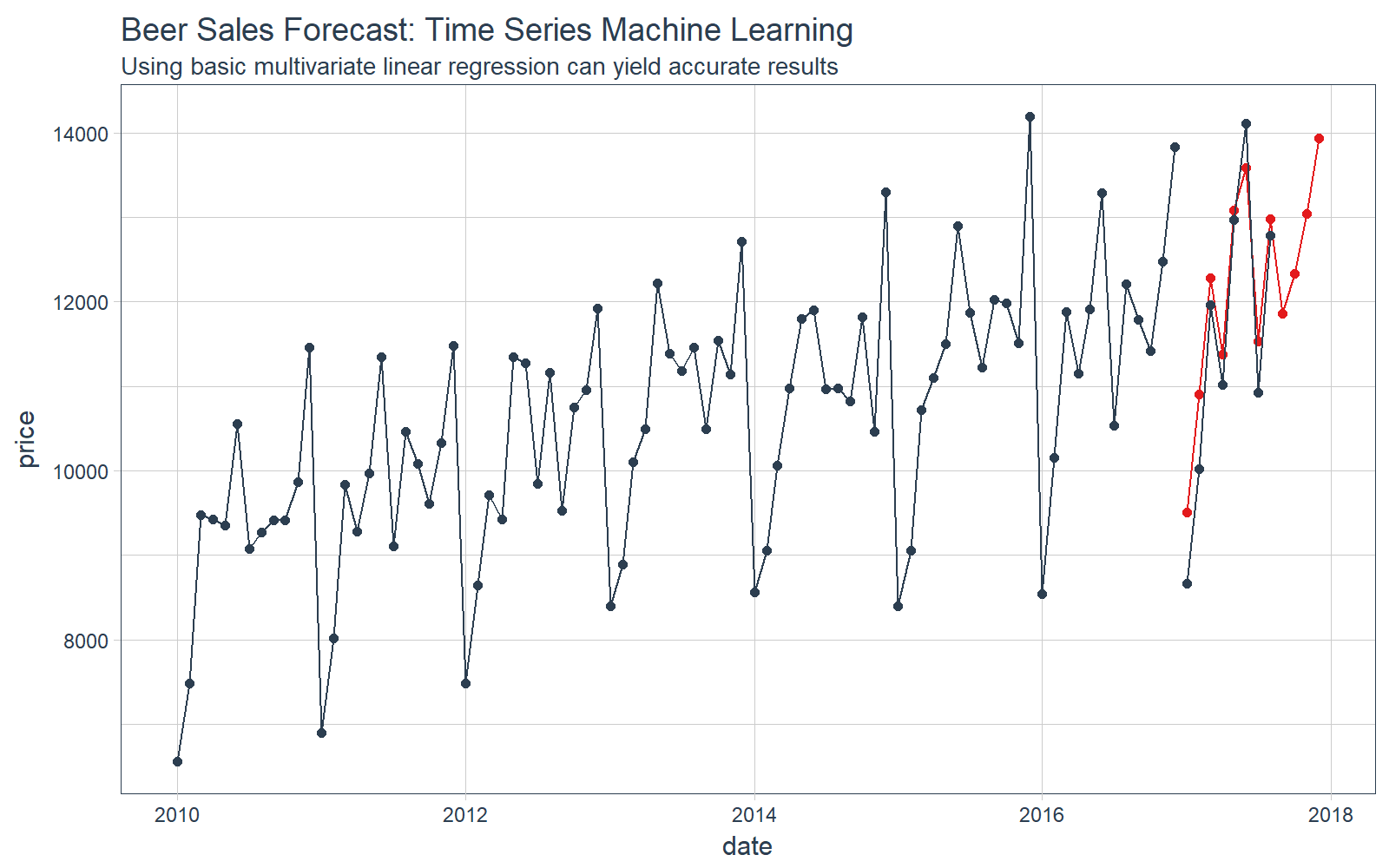
Visualize our forecast.
# Plot Beer Sales Forecast
beer_sales_tbl %>%
    ggplot(aes(x = date, y = price)) +
    # Training data
    geom_line(color = palette_light()[[1]]) +
    geom_point(color = palette_light()[[1]]) +
    # Predictions
    geom_line(aes(y = value), color = palette_light()[[2]], data = predictions_tbl) +
    geom_point(aes(y = value), color = palette_light()[[2]], data = predictions_tbl) +
    # Actuals
    geom_line(color = palette_light()[[1]], data = actuals_tbl) +
    geom_point(color = palette_light()[[1]], data = actuals_tbl) +
    # Aesthetics
    theme_tq() +
    labs(title = "Beer Sales Forecast: Time Series Machine Learning",
         subtitle = "Using basic multivariate linear regression can yield accurate results")
We can investigate the error on our test set (actuals vs predictions).
# Investigate test error
error_tbl <- left_join(actuals_tbl, predictions_tbl) %>%
    rename(actual = price, pred = value) %>%
    mutate(
        error     = actual - pred,
        error_pct = error / actual
        )
error_tbl
## # A tibble: 8 x 5
##         date actual      pred     error    error_pct
##       <date>  <int>     <dbl>     <dbl>        <dbl>
## 1 2017-01-01   8664  9509.122 -845.1223 -0.097544127
## 2 2017-02-01  10017 10909.189 -892.1891 -0.089067495
## 3 2017-03-01  11960 12281.835 -321.8352 -0.026909301
## 4 2017-04-01  11019 11378.678 -359.6777 -0.032641592
## 5 2017-05-01  12971 13080.710 -109.7099 -0.008458092
## 6 2017-06-01  14113 13583.471  529.5292  0.037520667
## 7 2017-07-01  10928 11529.085 -601.0854 -0.055004156
## 8 2017-08-01  12788 12984.939 -196.9386 -0.015400265
And we can calculate a few residuals metrics. The MAPE error is approximately 4.5% from the actual value, which is pretty good for a simple multivariate linear regression. A more complex algorithm could produce more accurate results.
# Calculating test error metrics
test_residuals <- error_tbl$error
test_error_pct <- error_tbl$error_pct * 100 # Percentage error

me   <- mean(test_residuals, na.rm=TRUE)
rmse <- mean(test_residuals^2, na.rm=TRUE)^0.5
mae  <- mean(abs(test_residuals), na.rm=TRUE)
mape <- mean(abs(test_error_pct), na.rm=TRUE)
mpe  <- mean(test_error_pct, na.rm=TRUE)

tibble(me, rmse, mae, mape, mpe) %>% glimpse()
## Observations: 1
## Variables: 5
## $ me   <dbl> -349.6286
## $ rmse <dbl> 551.7818
## $ mae  <dbl> 482.0109
## $ mape <dbl> 4.531821
## $ mpe  <dbl> -3.593805
Time series machine learning can produce exceptional forecasts. For those interested in learning more, we have a whole vignette dedicated to time series forecasting using timetk.
Part 2: Coercion
-
Problem: Switching between various time classes in R is painful and inconsistent.
-
Solution: tk_tbl, tk_xts, tk_zoo, tk_ts
tk_xts
We are starting with a tbl object. A disadvantage is that sometimes we would like to convert to an xts object to use xts-based functions from the numerous packages that deal with xts objects (xts, zoo, quantmod, etc).
We can easily convert to an xts object using tk_xts(). Notice that tk_xts() auto-detects the time-based column and uses its values as the index for the xts object.
# Coerce to xts
beer_sales_xts <- tk_xts(beer_sales_tbl)

# Show the first six rows of the xts object
beer_sales_xts %>%
    head()
##            price
## 2010-01-01  6558
## 2010-02-01  7481
## 2010-03-01  9475
## 2010-04-01  9424
## 2010-05-01  9351
## 2010-06-01 10552
We can also go from xts back to tbl. We tack on rename_index = "date" to have the index name match what we started with. This used to be very difficult. Notice that
tk_tbl(beer_sales_xts, rename_index = "date")
## # A tibble: 84 x 2
##          date price
##        <date> <int>
##  1 2010-01-01  6558
##  2 2010-02-01  7481
##  3 2010-03-01  9475
##  4 2010-04-01  9424
##  5 2010-05-01  9351
##  6 2010-06-01 10552
##  7 2010-07-01  9077
##  8 2010-08-01  9273
##  9 2010-09-01  9420
## 10 2010-10-01  9413
## # ... with 74 more rows
tk_ts
A number of packages use a different time class called ts. Probably the most popular is the forecast package. The advantage of using the tk_ts() function is two-fold:
- It’s consistent with the other
tk_ coercion functions so coercing back and forth is straightforward and easy.
- IMPORTANT: When
tk_ts() is used, the ts-object carries the original irregular time index (usually dates) as an index attribute. This makes keeping date and datetime information possible.
Here’s an example. We can use tk_ts() to convert to a ts object. Because the ts-based system only works with regular time series, we need to add the arguments start = 2010 and freq = 12.
# Coerce to ts
beer_sales_ts <- tk_ts(beer_sales_tbl, start = 2010, freq = 12)

# Show the calendar-printout
beer_sales_ts
##        Jan   Feb   Mar   Apr   May   Jun   Jul   Aug   Sep   Oct
## 2010  6558  7481  9475  9424  9351 10552  9077  9273  9420  9413
## 2011  6901  8014  9833  9281  9967 11344  9106 10468 10085  9612
## 2012  7486  8641  9709  9423 11342 11274  9845 11163  9532 10754
## 2013  8395  8888 10109 10493 12217 11385 11186 11462 10494 11541
## 2014  8559  9061 10058 10979 11794 11906 10966 10981 10827 11815
## 2015  8398  9061 10720 11105 11505 12903 11866 11223 12023 11986
## 2016  8540 10158 11879 11155 11916 13291 10540 12212 11786 11424
##        Nov   Dec
## 2010  9866 11455
## 2011 10328 11483
## 2012 10953 11922
## 2013 11139 12709
## 2014 10466 13303
## 2015 11510 14190
## 2016 12482 13832
There are two ways we can go back to tbl:
- Just coerce back using
tk_tbl() and we get the “regular” index as YEARMON data type from zoo.
- If the object was created with
tk_ts() and has a timetk_index, we can coerce back using tk_tbl(timetk_index = TRUE) and we get the original “irregular” index as Date data type.
Method 1: We go back to tbl. Note that the date column is YEARMON class.
tk_tbl(beer_sales_ts, rename_index = "date")
## # A tibble: 84 x 2
##             date price
##    <S3: yearmon> <int>
##  1      Jan 2010  6558
##  2      Feb 2010  7481
##  3      Mar 2010  9475
##  4      Apr 2010  9424
##  5      May 2010  9351
##  6      Jun 2010 10552
##  7      Jul 2010  9077
##  8      Aug 2010  9273
##  9      Sep 2010  9420
## 10      Oct 2010  9413
## # ... with 74 more rows
Method 2: We go back to tbl but specify timetk_idx = TRUE to return original DATE or DATETIME information.
First, you can check to see if the ts-object has a timetk index with has_timetk_idx().
# Check for timetk index.
has_timetk_idx(beer_sales_ts)
## [1] TRUE
If TRUE, then specify timetk_idx = TRUE during the tk_tbl() coercion. See that we now have “date” data type. This was previously very difficult to do.
# If timetk_idx is present, can get original dates back
tk_tbl(beer_sales_ts, timetk_idx = TRUE, rename_index = "date")
## # A tibble: 84 x 2
##          date price
##        <date> <int>
##  1 2010-01-01  6558
##  2 2010-02-01  7481
##  3 2010-03-01  9475
##  4 2010-04-01  9424
##  5 2010-05-01  9351
##  6 2010-06-01 10552
##  7 2010-07-01  9077
##  8 2010-08-01  9273
##  9 2010-09-01  9420
## 10 2010-10-01  9413
## # ... with 74 more rows
Next Steps
We’ve only scratched the surface of timetk. There’s more to learn including working with time series indices and making future indices. Here are a few resources to help you along the way:
Announcements
We have a busy couple of weeks. In addition to Demo Week, we have:
DataTalk
On Thursday, October 26 at 7PM EST, Matt will be giving a FREE LIVE #DataTalk on Machine Learning for Recruitment and Reducing Employee Attrition. You can sign up for a reminder at the Experian Data Lab website.
EARL
On Friday, November 3rd, Matt will be presenting at the EARL Conference on HR Analytics: Using Machine Learning to Predict Employee Turnover.
Courses
Based on recent demand, we are considering offering application-specific machine learning courses for Data Scientists. The content will be business problems similar to our popular articles:
The student will learn from Business Science how to implement cutting edge data science to solve business problems. Please let us know if you are interested. You can leave comments as to what you would like to see at the bottom of the post in Disqus.
About Business Science
Business Science specializes in “ROI-driven data science”. Our focus is machine learning and data science in business applications. We help businesses that seek to add this competitive advantage but may not have the resources currently to implement predictive analytics. Business Science works with clients primarily in small to medium size businesses, guiding these organizations in expanding predictive analytics while executing on ROI generating projects. Visit the Business Science website or contact us to learn more!