BizSci Package Updates: Formerly timekit... Now timetk :)
Written by Matt Dancho

We have several announcements regarding Business Science R packages. First, as of this week the R package formerly known as timekit has changed to timetk for time series tool kit. There are a few “breaking” changes because of the name change, and this is discussed further below. Second, the sweep and tidyquant packages have several improvements, which are discussed in detail below. Finally, don’t miss a beat on future news, events and information by following us on social media.
timetk
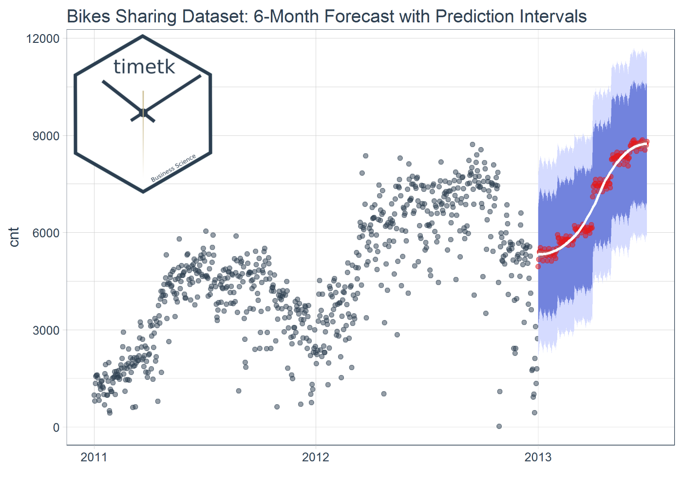
The timetk package (formerly timekit) is a relatively new package that is aimed at assisting users with working with time series in R. It helps users switch back and forth between time based “tibbles” (tidy data frames with dates or date times) and the other time series objects in R (xts, zoo, ts, etc). Equally important, timetk includes functions that help setup time series for data mining and machine learning. Here’s an example from Vignette #4: Forecasting Using a Time Series Signature with timetk:
Why the name change? The name change was made to help differentiate from timekit.io. It was in both parties best interest to differentiate, which is less confusing to users of both organizations’ software.
The primary change is to the name of the package, and most functions are the same. There are however a few “breaking changes” that are a result of the name change. We made the transition very simple. All you need to do to refactor is “Ctrl+F” or “Cmd+F” and find and replace “timekit” with “timetk”, and everything will work. We promise!
Here’s some examples of the changes. Notice the functions are all the same. Only changes are related to “timekit”.
-
The function has_timekit_index() now changes to has_timetk_index(). This function is used to detect if a ts object has a “timetk index” (non-regularized date or datetime, which are present in ts objects coerced with tk_ts()). Again, just refactor and you will be fine.
-
Functions with the boolean argument timekit_idx have the argument changed to timetk_idx. Examples include tk_index(timetk_idx = TRUE) and tk_tbl(timetk_idx = TRUE). The timetk_idx argument enables retrieving a non-regularized date or datetime series rather than the regularized time series typically present in ts objects. Note that this only is applicable if the tk_ts() coercion function is used during initial coercion to a ts object. Refer to the Vignette #1: Time Series Coercion Using timetk for more details.
That’s it. It should be very easy to make the transition to timetk via a simple refactor. Please let us know if you have any issues. You can contact us at [email protected] or via social media below.
sweep
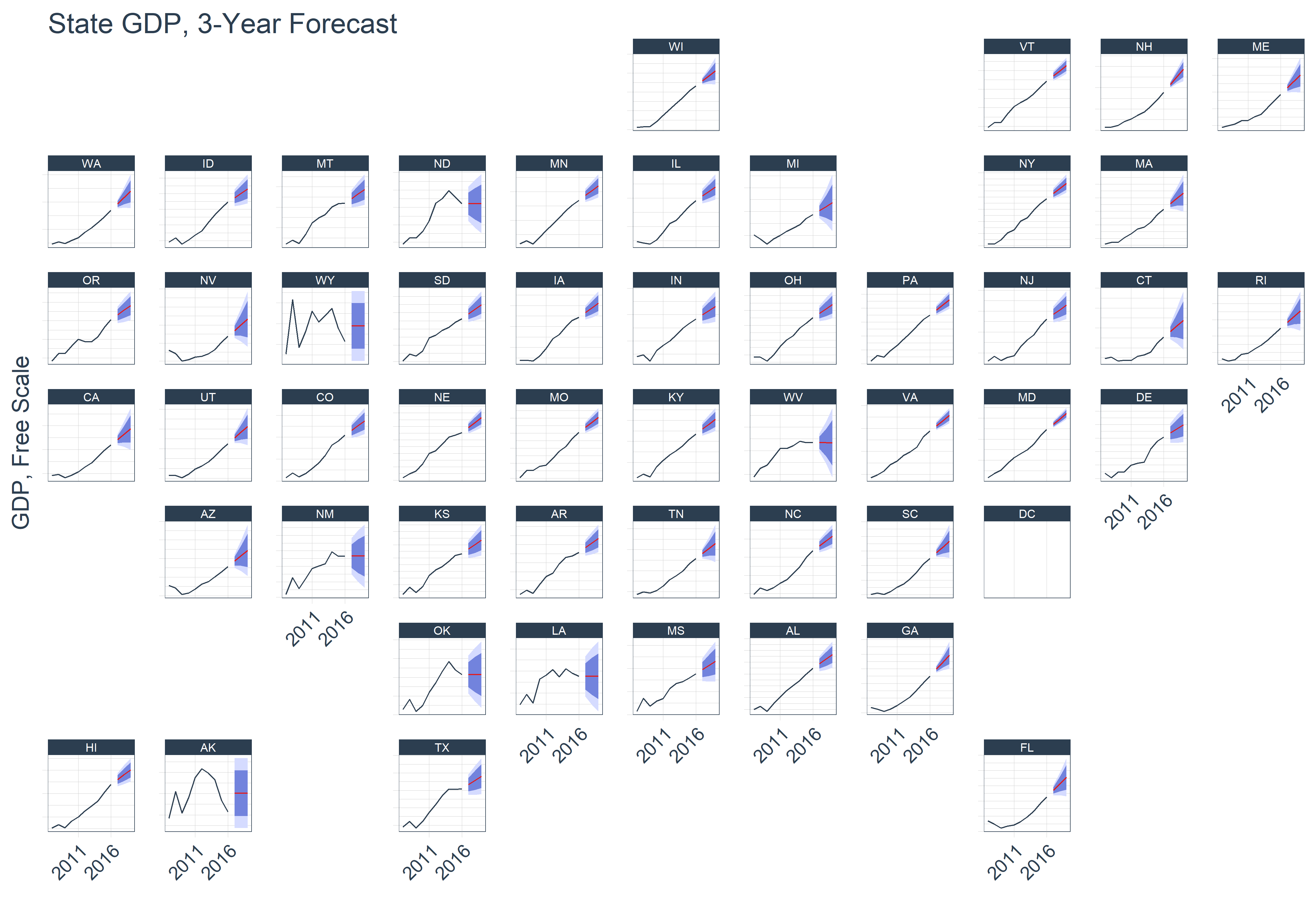
The sweep package is designed to “tidy” the model and forecast output of packages that use the ts system. The most popular example is the forecast package. The package uses broom-style tidiers (sw_tidy, sw_glance, sw_augment and sw_sweep) to convert the output to “tibbles”. Here’s an example from our recent sweep blog post where we collected GDP for each US state and plotted “tidy” ARIMA forecasts.
The main addition to sweep v0.2.0 is support for the robets package. The addition was user supplied via pull request (thanks Joel Gombin). We highly encourage users interested in converting models in other ts-based packages to “tidy” output to submit pull requests! Let us know if you are interested in helping.
The other main change is to the sw_sweep() function, which is used to convert forecast objects to “tidy” data frames. Because it uses timetk under the hood to convert the ts object time series to date or datetime, we changed the timekit_idx argument to timetk_idx. Again, just refactor to change to the sw_sweep(timetk_idx) argument. For more information, refer to the Introduction to sweep Vignette .
tidyquant
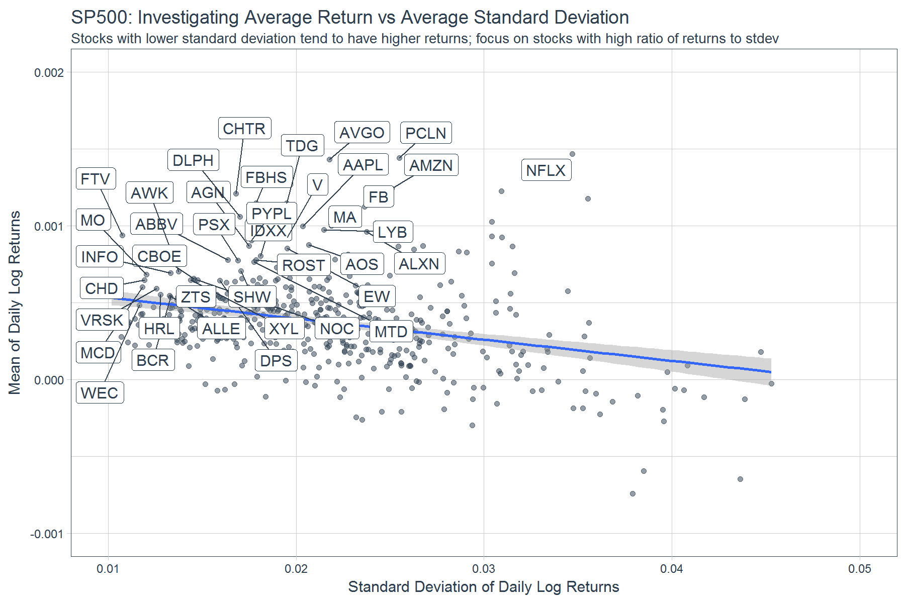
The tidyquant package bridges a gap between the “tidyverse” and many of the financial and time series packages that depend on the xts and zoo time series objects. The main benefit is the scale-ability to perform grouped operations, which can be difficult in the xts system when managing multiple time series. Here’s a simple example to show why you might consider using tidyquant. The script below retrieves the past 10-years of stock prices for every stock in the SP500, then calculates the average and standard deviation of the daily returns.
# Analyzing every stock in SP500
library(tidyquant)
sp500_analysis <- tq_index("SP500") %>%  # Get stock list
    # Get stock prices for each stock in list
    tq_get() %>%
    # Group for grouped analysis
    group_by(symbol) %>%
    # Convert from daily prices to daily log(returns)
    tq_transmute(
        select      = adjusted,
        mutate_fun  = periodReturn,
        period      = "daily",
        type        = "log",
        col_rename  = "daily.log.return"
    ) %>%
    # Calculate mean and stdev of log returns
    summarize(
        dlr_mean = mean(daily.log.return),
        dlr_sd   = sd(daily.log.return)
    )
Here’s a useful plot you can make with the data. An investor can easily focus on stocks that have lower risk and higher reward metrics.
library(ggrepel)

# Plot mean vs standard deviation of daily log returns
sp500_analysis %>%
    ggplot(aes(x = dlr_sd, y = dlr_mean)) +
    # Data viz
    geom_point(color = palette_light()[[1]], alpha = 0.5) +
    geom_smooth(method = "lm") +
    # Show high ratio of returns to volatility
    geom_label_repel(
        aes(label = symbol),
        color = palette_light()[[1]],
        data  = subset(sp500_analysis, dlr_mean / dlr_sd > .04)
    ) +
    # Aethetics
    scale_x_continuous(limits = c(0.01, 0.05)) +
    scale_y_continuous(limits = c(-0.001, 0.002)) +
    labs(
        title = "SP500: Investigating Average Return vs Average Standard Deviation",
        subtitle = "Stocks with lower standard deviation tend to have higher returns; focus on stocks with high ratio of returns to stdev",
        x = "Standard Deviation of Daily Log Returns",
        y = "Mean of Daily Log Returns"
    ) +
    theme_tq()
What are the changes? There’s two main changes in tidyquant v0.5.2.
First, tq_index(), the function used to get stock indexes such as SP500, DOW, and RUSSELL2000 now collects its data from SPDRs. The tq_index_options are:
# List of indexes available for download, supply desired option to tq_index()
tq_index_options()
## [1] "RUSSELL1000" "RUSSELL2000" "RUSSELL3000" "DOW"
## [5] "DOWGLOBAL"   "SP400"       "SP500"       "SP600"
## [9] "SP1000"
The return from tq_index() now include weight, sector, and shares_held from the associated SPDR.
# New source for index
library(tidyquant)
tq_index("SP500") %>%
    head()
| symbol |
company |
weight |
sector |
shares_held |
| AAPL |
Apple Inc. |
0.0377152 |
Information Technology |
59372276 |
| MSFT |
Microsoft Corporation |
0.0269475 |
Information Technology |
87913770 |
| AMZN |
Amazon.com Inc. |
0.0196867 |
Consumer Discretionary |
4517403 |
| FB |
Facebook Inc. Class A |
0.0184511 |
Information Technology |
26915296 |
| JNJ |
Johnson & Johnson |
0.0166280 |
Health Care |
30675892 |
| XOM |
Exxon Mobil Corporation |
0.0160500 |
Energy |
48243920 |
Second, the tidyquant::as_tibble() and tidyquant::as_xts() functions are now deprecated. These were used to convert between xts and time-based tibble objects. You can still use them (for now), but you will receive a warning. Rather, you should transition to the more robust timetk tk_tbl() and tk_xts() functions, which do the same thing in a more automated way.
# Create some prices as time-based tibble
set.seed(8357)
prices_tbl <- tibble(
    date = seq.Date(from = as.Date("2017-01-01"), to = as.Date("2017-01-10"), by = "day"),
    price = seq(from = 100, 120, length.out = 10) + rnorm(n = 10)
)
Use timetk::tk_xts() to coerce any time based object to xts. Dates are converted and dropped automatically. Use silent = TRUE to eliminate messages describing date column being dropped and converted to index. This replaces tidyquant::as_xts() which only worked with tibble objects.
library(timetk)

# Use tk_xts() to easily coerce to xts
prices_xts <- tk_xts(prices_tbl, silent = TRUE)
prices_xts
##                price
## 2017-01-01  99.22609
## 2017-01-02 100.98272
## 2017-01-03 103.50840
## 2017-01-04 105.20828
## 2017-01-05 110.83621
## 2017-01-06 110.63730
## 2017-01-07 113.96259
## 2017-01-08 115.70832
## 2017-01-09 117.94495
## 2017-01-10 120.25419
class(prices_xts)
## [1] "xts" "zoo"
Use timetk::tk_tbl() to coerce any time based object to tibble. This replaces tidyquant::as_tibble() which only worked with xts objects.
# Use tk_tbl() to easily coerce back to tbl
tk_tbl(prices_xts, rename_index = "date", silent = TRUE)
## # A tibble: 10 x 2
##          date     price
##        <date>     <dbl>
##  1 2017-01-01  99.22609
##  2 2017-01-02 100.98272
##  3 2017-01-03 103.50840
##  4 2017-01-04 105.20828
##  5 2017-01-05 110.83621
##  6 2017-01-06 110.63730
##  7 2017-01-07 113.96259
##  8 2017-01-08 115.70832
##  9 2017-01-09 117.94495
## 10 2017-01-10 120.25419
About Business Science
We have a full suite of data science services to supercharge your organizations financial and business performance! For example, our experienced data scientists reduced a manufacturer’s sales forecasting error by 50%, which led to improved personnel planning, material purchasing and inventory management.
How do we do it? With team-based data science: Using our network of data science consultants with expertise in Marketing, Forecasting, Finance and more, we pull together the right team to get custom projects done on time, within budget, and of the highest quality. Learn about our data science services or contact us!
We are growing! Let us know if you are interested in joining our network of data scientist consultants. If you have expertise in Marketing Analytics, Data Science for Business, Financial Analytics, Forecasting or Data Science in general, we’d love to talk. Contact us!