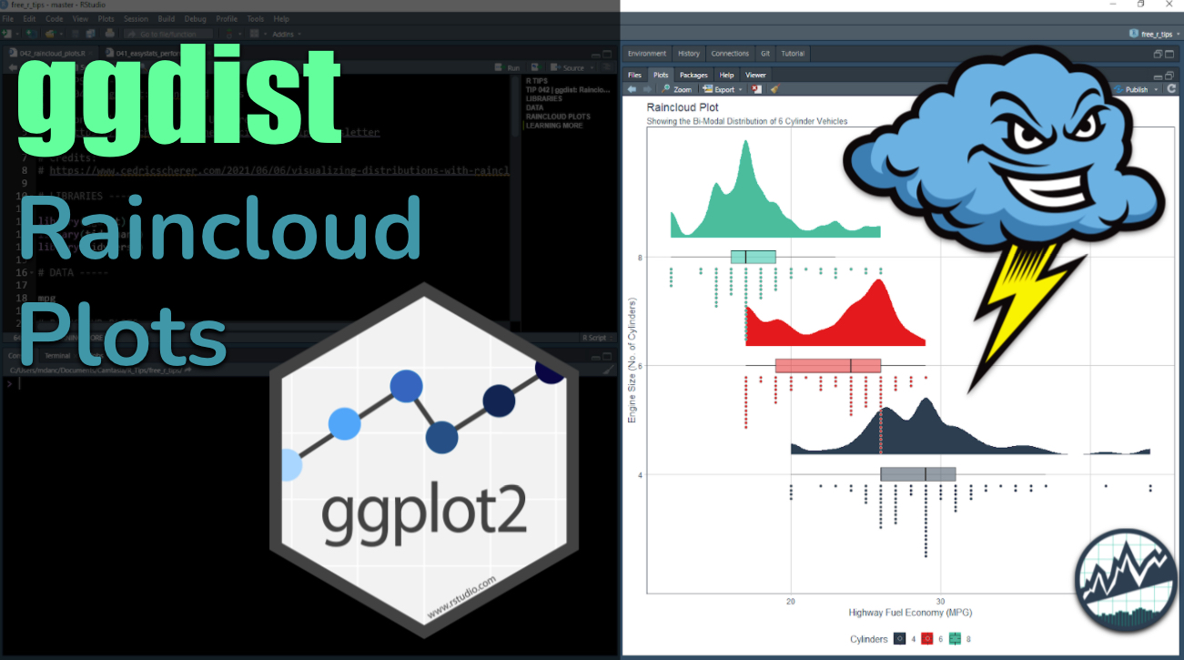
ggdist: Make a Raincloud Plot to Visualize Distribution in ggplot2
Written by Matt Dancho
One of the most important things a data scientist can do that will uncover business insights is to Visualize distributions.
And, this is something I had a hard time with. But I recently found an easy solution.
I discovered the ggdist package that made visualizing distributions a breeze. It’s a ggplot2 extension that is made for visualizing distributions and uncertainty. Here’s what you’ll discover in the next 5 minutes:
- Discover how
ggdist can be used to make a raincloud plot.
- BONUS: Get 5 plotting tips that even beginners can implement to make professional raincloud plots
SPECIAL ANNOUNCEMENT: AI for Data Scientists Workshop on December 18th
Inside the workshop I’ll share how I built a SQL-Writing Business Intelligence Agent with Generative AI:
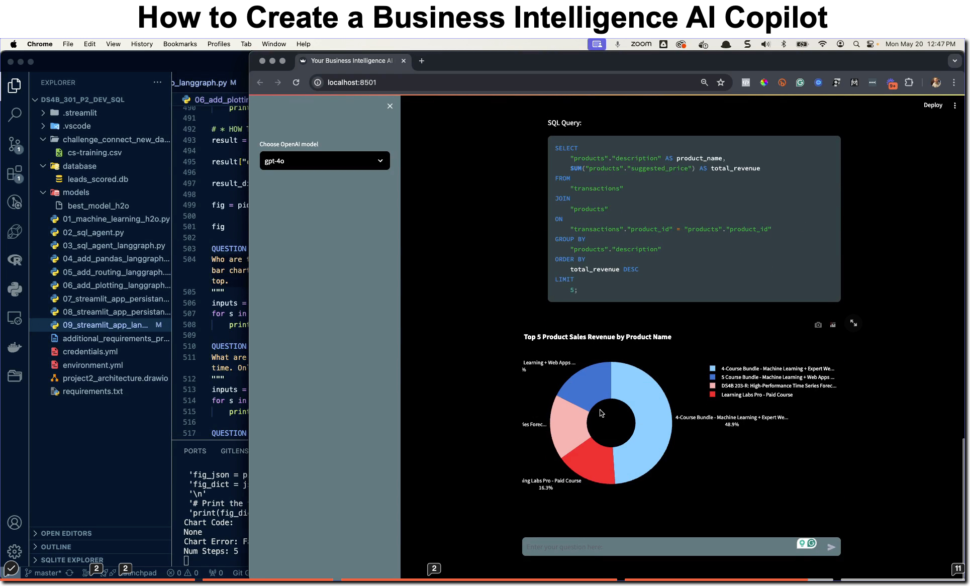
What: GenAI for Data Scientists
When: Wednesday December 18th, 2pm EST
How It Will Help You: Whether you are new to data science or are an expert, Generative AI is changing the game. There’s a ton of hype. But how can Generative AI actually help you become a better data scientist and help you stand out in your career? I’ll show you inside my free Generative AI for Data Scientists workshop.
Price: Does Free sound good?
How To Join: 👉 Register Here
R-Tips Weekly
This article is part of R-Tips Weekly, a weekly video tutorial that shows you step-by-step how to do common R coding tasks.
Here are the links to get set up. 👇
This Tutorial Is Available In Video
I have a companion video tutorial that shows even more secrets (plus mistakes to avoid). And, I’m finding that a lot of my students prefer the dialogue that goes along with coding. So check out this video to see me running the code in this tutorial. 👇
What is a Raincloud Plot?
The Raincloud Plot is a visualization that produces a half-density to a distribution plot. It gets the name because the density plot is in the shape of a “raincloud”. The raincloud plot enhances the traditional box plot by highlighting multiple modalities (an indicator that groups may exist). The boxplot does not show where densities are clustered, but the raincloud plot does!
Raincloud Plot (We'll make in this tutorial)
We’ll go through a short tutorial to get you up and running with ggdist to make a raincloud plot.
Raincloud Plots with ggdist [Tutorial]
This tutorial showcases the awesome power of ggdist for visualizing distributions.
Tutorial Credits
This tutorial wouldn’t be possible without another tutorial, Visualizing Distributions with Raincloud Plots by Cédric Scherer. Cédric truly a ggplot2 master. Follow Cédric Scherer on Twitter to learn more about his excellent visualization work.
Ever forget which R package to use?
Ever forget which R package to use? Or which tidyverse function to apply? Me too.
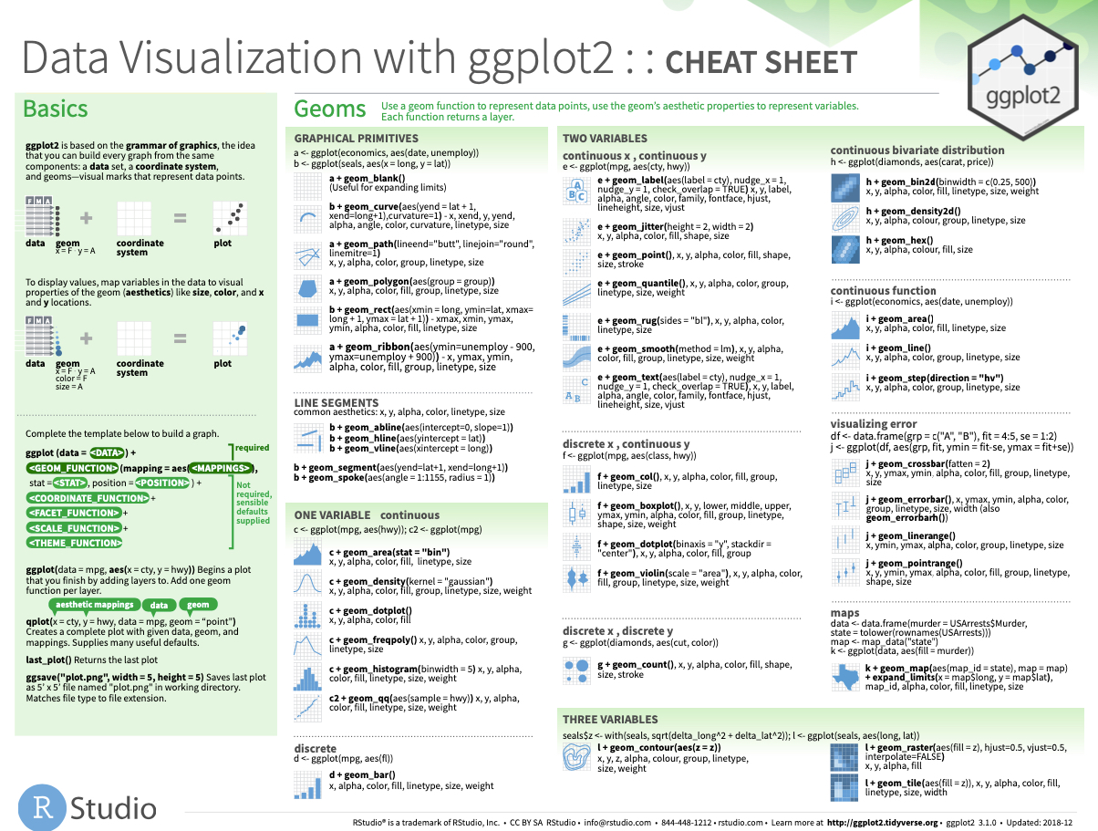
That’s why I made my ultimate R cheat sheet. Here’s how to use it for ggplot2 visualizations and plotting.
Step 1: Download the Ultimate R Cheat Sheet.
Step 2: Then Click the “CS” hyperlink to “ggplot2”.
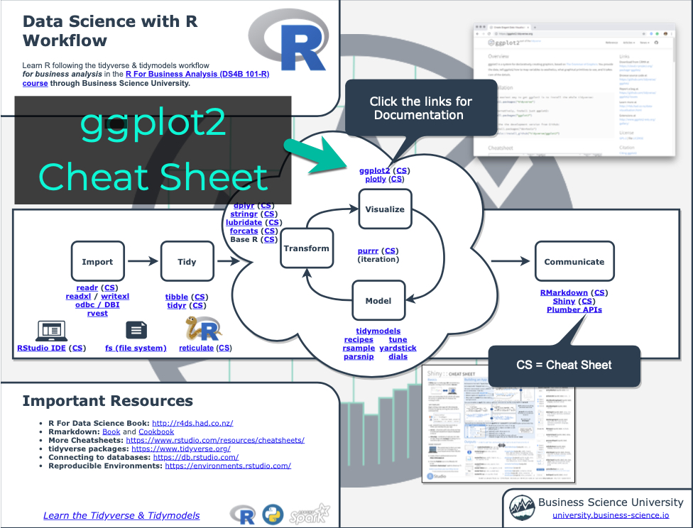
Step 3: Reference the ggplot2 cheat sheet. This shows you the core plotting functions available in the ggplot library. Now you can use these any time you need to make a visualization with ggplot2.
Pretty handy. Now let’s get going…
Load the Libraries and Data
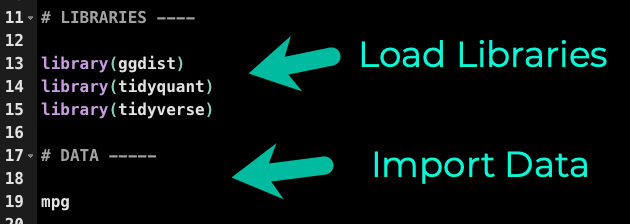
First, run this code to:
- Load Libraries: Load
ggdist, tidyquant, and tidyverse.
- Import Data: We’re using the
mpg dataset that comes with ggplot2.
Get the code.
Raincloud Plot: Using ggplot2 + ggdist
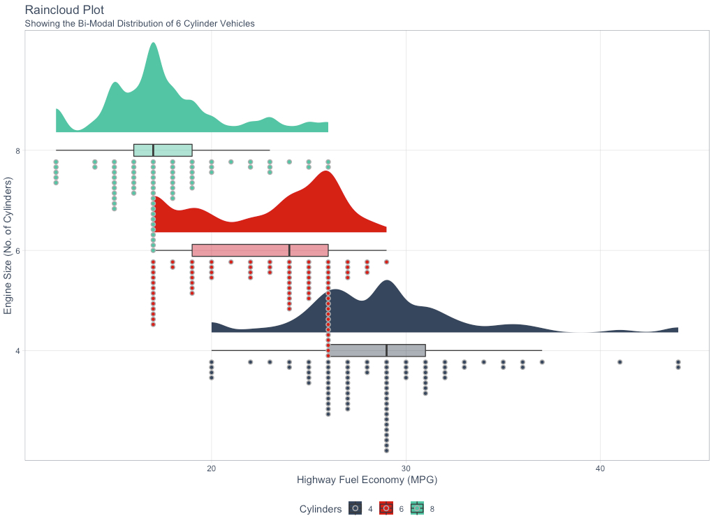
Next, we’ll make a Raincloud plot that highlights the distribution of Vehicle Fuel Economy (MPG) by Engine Size (Number of Cylinders). We’ll combine ggplot2 and ggdist through 5 plotting tips that even beginners can implement.
Tip 1: Make the ggplot2 canvas
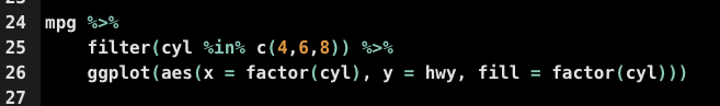
The first step is to make the ggplot2 canvas. We:
- Prep the Data: Using
filter() to isolate the most common (frequent) vehicle engine sizes
- Map the columns: Using
ggplot(), we map the cyl and hwy column. We also make a transformation to convert a numeric cyl column to a discrete cyl column with factor().
Get the code.
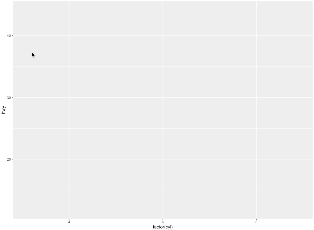
This produces a blank plot, which is the first layer. You can see that the x-axis is labeled “factor(cyl)” and the y-axis is “hwy” indicating the data has been mapped to the visualization.
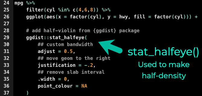
Tip 2: Add the Rainclouds with stat_halfeye())
Next, we add our first geometry layer using ggdist::stat_halfeye(). This produces a Half Eye visualization, which is contains a half-density and a slab-interval. We remove the slab interval by setting .width = 0 and point_colour = NA. The half-density remains.
Get the code.
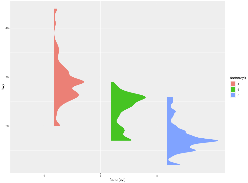
And here’s the output. We can see the half-denisty distributions for fuel economy (hwy) by engine size (cyl).
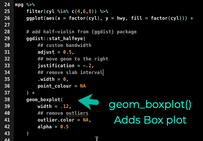
Tip 3: Add the Boxplot with geom_boxplot()
Next, add the second geometry layer using ggplot2::geom_boxplot(). This produces a narrow boxplot. We reduce the width and adjust the opacity.
Get the code.
And here’s the output. We now have a boxplot and half-density. We can see how the distributions vary compared to the median and inner-quartile range.
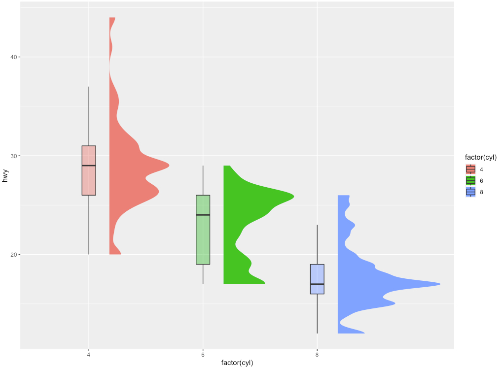
Tip 4: Add the Dot Plots with stat_dots()
Next, add the third geometry layer using ggdist::stat_dots(). This produces a half-dotplot, which is similar to a histogram that indicates the number of samples (number of dots) in each bin. We select side = "left" to indicate we want it on the left-hand side.
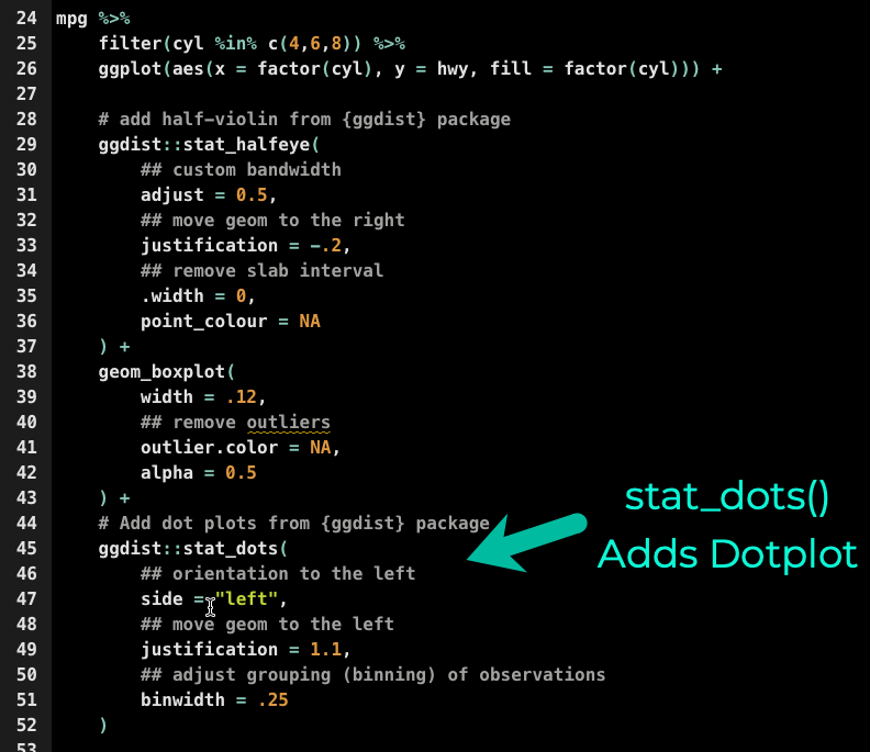
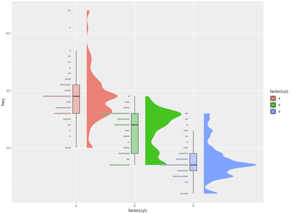
Get the code.
And here’s the output. We now have the three main geometries completed.
Tip 5: Making the plot look professional
We can clean up our plot with a professional-looking theme using tidyquant::theme_tq(). We’ll also rotate it with coord_flip() to give it the raincloud appearance.
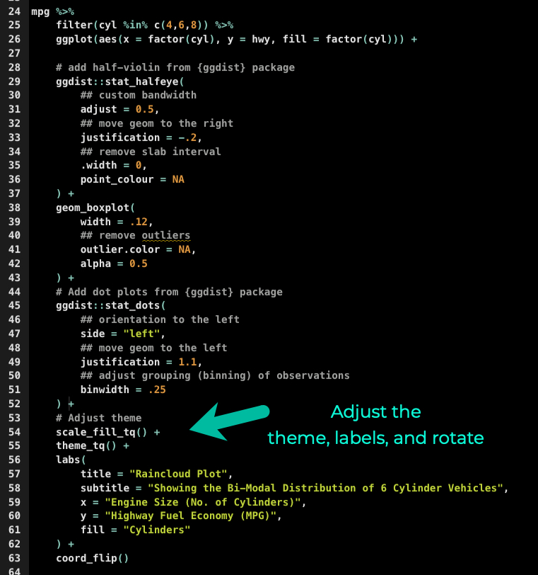
Get the code.
We’ve just finalized our plot. We can see clearly that the distribution of the 6-cylinder is bi-modal, something you can’t tell with an ordinary boxplot. We should investigate why there are so many dots in 6-cylinder with low highway-fuel economy. We’ll save that for another R-Tip.

Conclusions
You just learned how to make Raincloud Plots with ggdist. But, there’s a lot more to visualization.
It’s critical to learn how to visualize with ggplot2, which is the premier framework for data visualization in R.
If you’d like to learn ggplot2, data visualizations, and data science for business with R, then read on. 👇
Need to advance your business data science skills?
I’ve helped 6,107+ students learn data science for business from an elite business consultant’s perspective.
I’ve worked with Fortune 500 companies like S&P Global, Apple, MRM McCann, and more.
And I built a training program that gets my students life-changing data science careers (don’t believe me? see my testimonials here):
6-Figure Data Science Job at CVS Health ($125K)
Senior VP Of Analytics At JP Morgan ($200K)
50%+ Raises & Promotions ($150K)
Lead Data Scientist at Northwestern Mutual ($175K)
2X-ed Salary (From $60K to $120K)
2 Competing ML Job Offers ($150K)
Promotion to Lead Data Scientist ($175K)
Data Scientist Job at Verizon ($125K+)
Data Scientist Job at CitiBank ($100K + Bonus)
Whenever you are ready, here’s the system they are taking:
Here’s the system that has gotten aspiring data scientists, career transitioners, and life long learners data science jobs and promotions…
Join My 5-Course R-Track Program Now!
(And Become The Data Scientist You Were Meant To Be...)
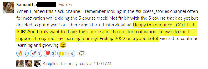
P.S. - Samantha landed her NEW Data Science R Developer job at CVS Health (Fortune 500). This could be you.