Forecasting Many Time Series (Using NO For-Loops)
Written by Matt Dancho
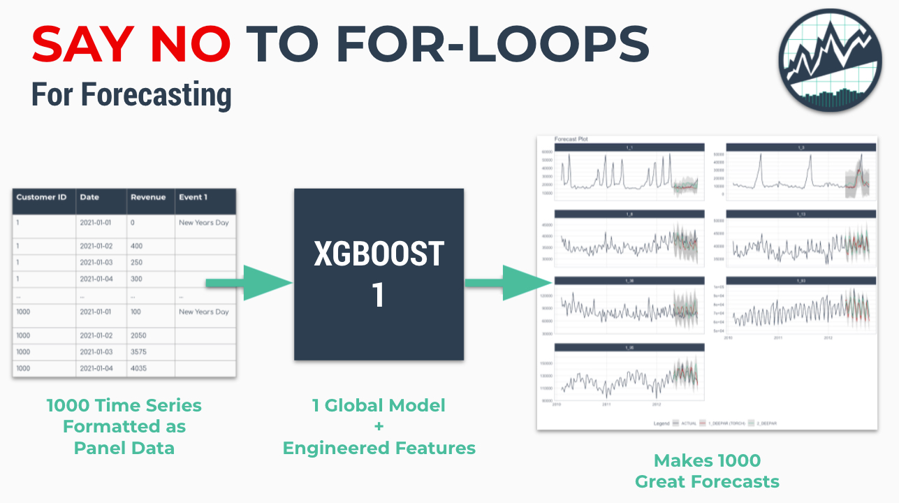
Spending too much time on making iterative forecasts? I’m super excited to introduce the new panel data forecasting functionality in modeltime. It’s perfect for forecasting many time series at once without for-loops saving you time ⏱️ and aggravation 😞. Just say NO to for-loops for forecasting.
Fitting many time series can be an expensive process. The most widely-accepted technique is to iteratively run an ARIMA model on each time series in a for-loop.
Times are changing. Organizations now need 1000’s of forecasts. Think 1000s of customers, products, and complex hierarchical data.
In this tutorial:
-
We’ll explain new techniques involving Global Models and Panel Data for dealing with many time series.
-
We’ll then provide an introductory tutorial using modeltime 0.7.0 new features (now available on CRAN 🎉) for modeling time series as Panel Data to make forecasts without for-loops.
If you like what you see, I have an Advanced Time Series Course where you will learn the foundations of the growing Modeltime Ecosystem.
First, here’s a quick overview of the Modeltime Forecasting Ecosystem that unlocks tidymodels (similar to scikit learn but in R).
What is Modeltime?
A growing ecosystem for tidymodels forecasting
Modeltime is part of a growing ecosystem of forecasting packages. Modeltime integrates tidymodels for forecasting at scale. The ecosystem contains:
And several new community-contributed modeltime extension packages have emerged including: boostime, bayesmodels, garchmodels, and sknifedatar
Problem: Forecasting with For-Loops is Not Scalable
Time series data is increasing at an exponential rate. Organization-wide forecasting demands have changed from top-level to bottom-level forecasting, which has increased the number of forecasts that need to be made from the range of 1-100 to the range of 1,000-10,000.
Think of forecasting by customer for an organization that has 10,000 customers. It becomes a challenge to make these forecasts one at a time in an iterative approach. As that organization grows, moving from 10,000 to 100,000 customers, forecasting with an iterative approach is not scalable.
Modeltime has been designed to take a different approach using Panel Data and Global Models (more on these concepts shortly). Using these approaches, we can dramatically increase the scale at which forecasts can be made. Prior limitations in the range of 1,000 to 10,000 forecasts become managable. Beyond is also possible with clustering techniques and making several panel models. We are only limited by RAM, not modeling time.
Before we move on, we need to cover two key concepts:
- Panel Data
- Global Models
What are Panel Data and Global Models?
In it’s simplest form, Panel Data is a time series dataset that has more than one series. Each time series is stacked row-wise (on-top) of each other.
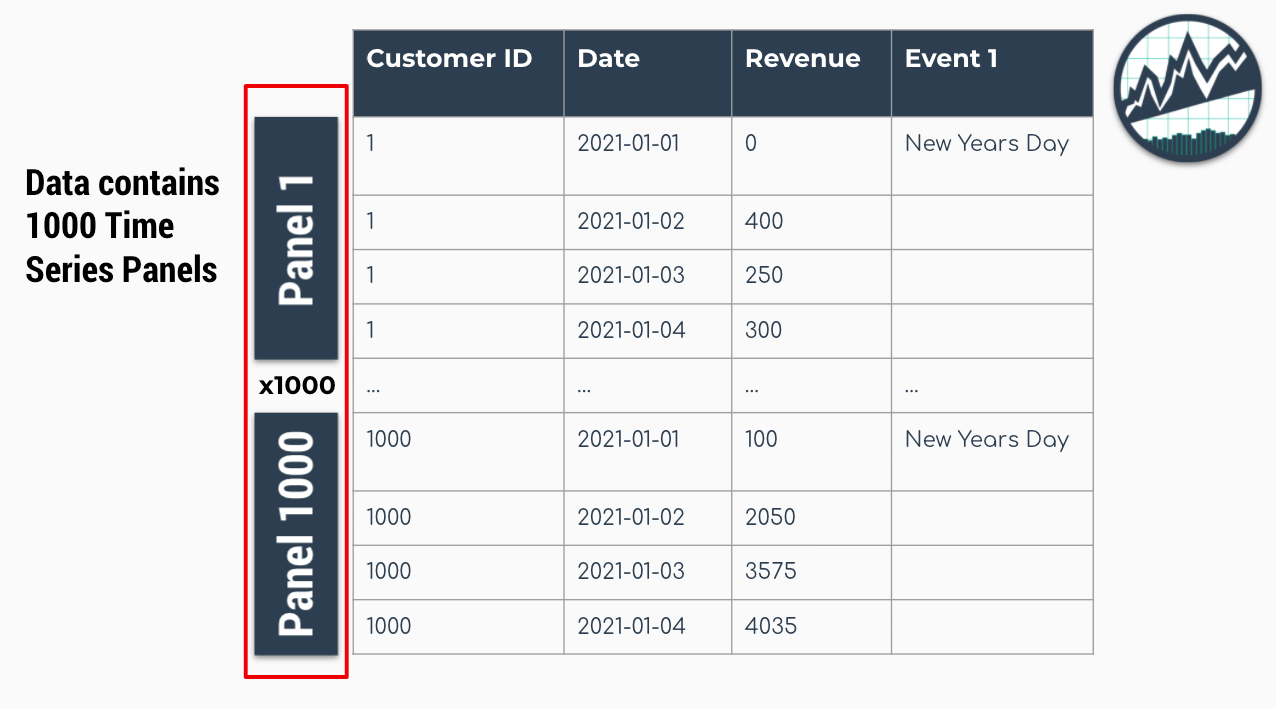
The Panel Data Time Series Format
Traditional modeling techniques like ARIMA can only be used on one time series at a time. The widely accepted forecasting approach is to iterate through each time series producing a unique model and forecast for each time series identifier. The downside with this approach is that it’s expensive when you have many time series. Think of the number of products in a database. As the number of time series approaches the range of 1000-10,000, the iterative approach becomes unscalable as for-loops run endlessly and errors can grind your analysis to a hault.
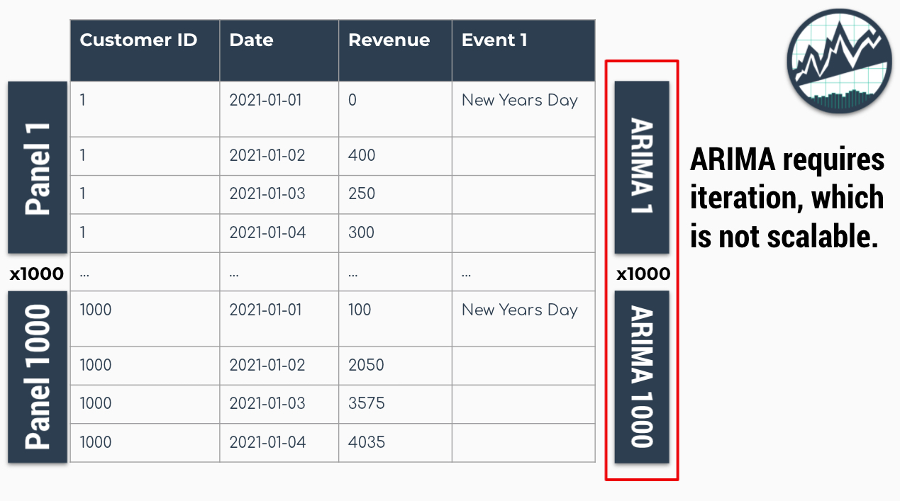
Problem: 1000 ARIMA Models Needed for 1000 Time Series
Global Models are alternatives to the iterative approach. A Global Model is a single model that forecasts all time series at once. Global Models are highly scalable, which solves the problem of 1-10,000 time series. An example is an XGBoost Model, which can determine relationships for all 1000 time series panels with a single model. This is great: No For-Loops!
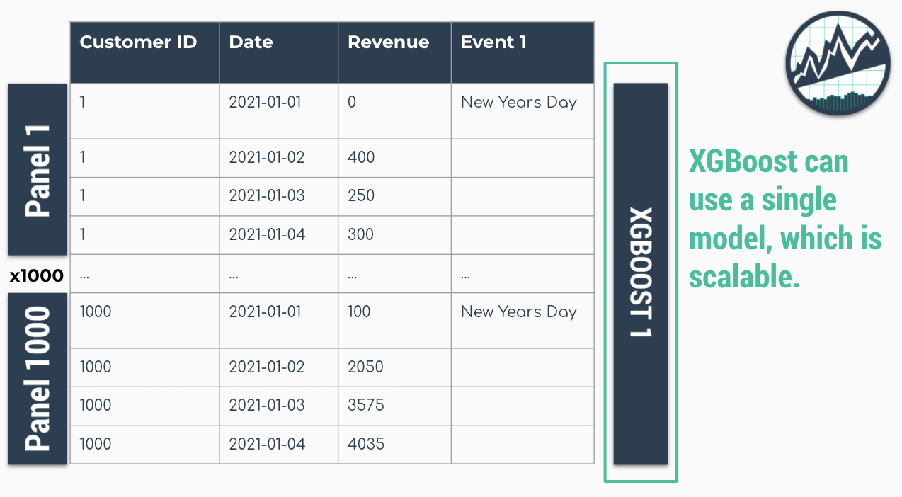
Solution: A Single XGBOOST Model can Model 1000 Time Series leaves you waiting for hours ⏳...
The downside is that an global model approach can be less accurate than the iterative approach. To improve accuracy, feature engineering and localized model selection by time series identifier become critical to large-scale forecasting success. If interested, I teach proven feature engineering techniques in my Time Series Forecasting Course.
Say No to For-Loops
If you’re tired of waiting for ARIMA models to finish, then maybe it’s time to say NO to for-loops and give modeltime a try.
Forecast using Global Models and Panel Data with Modeltime for a 1000X Speed-up
While Modeltime can perform iterative modeling, Modeltime excels at forecasting at scale without For-Loops using:
-
Global Modeling: Global model Machine Learning and Deep Learning strategies using the Modeltime Ecosystem (e.g. modeltime, modeltime.h2o, and modeltime.gluonts).
-
Panel Data: Tidy data that is easy to work with if you are familiar with the tidyverse and tidymodels.
-
Feature Engineering: Developing calendar features, lagged features, and other time-based, window-based, and sequence-based features using timetk.
-
Multi-Forecast Visualization: Visualizing multiple local time series forecasts at once.
-
Global and Localized Accuracy Reporting: Generating out-of-sample accuracy both globally and at a local level by time series identifier (available in modeltime >= 0.7.0)
-
Global and Localized Confidence Intervals Reporting: Generating out-of-sample confidence intervals both globally and at a local level by time series identifier (available in modeltime >= 0.7.0)
Once you learn these concepts, you can achieve speed-ups of 1000X or more. We’ll showcase several of these features in our tutorial on forecasting many time series without for-loops.
Tutorial on Forecasting Many Time Series (Without For-Loops)
We’ll cover a short tutorial on Forecasting Many Time Series (Without For-Loops).
Load Libraries
First, load the following libraries.
library(tidymodels)
library(modeltime)
library(tidyverse)
library(timetk)
Collect data
Next, collect the walmart_sales_weekly dataset. The dataset consists of 1001 observations of revenue generated by a store-department combination on any given week. It contains:
- 7 Time Series Groups denoted by the “ID” column
- The data is structured in Panel Data format
- The time series groups will be modeled with a single Global Model
data <- walmart_sales_weekly %>%
    select(id, Date, Weekly_Sales) %>%
    set_names(c("ID", "date", "value"))

data
## # A tibble: 1,001 x 3
##    ID    date        value
##    <fct> <date>      <dbl>
##  1 1_1   2010-02-05 24924.
##  2 1_1   2010-02-12 46039.
##  3 1_1   2010-02-19 41596.
##  4 1_1   2010-02-26 19404.
##  5 1_1   2010-03-05 21828.
##  6 1_1   2010-03-12 21043.
##  7 1_1   2010-03-19 22137.
##  8 1_1   2010-03-26 26229.
##  9 1_1   2010-04-02 57258.
## 10 1_1   2010-04-09 42961.
## # … with 991 more rows
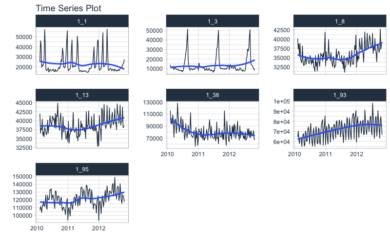
Visualize the Data
From visualizing, the weekly department revenue patterns emerge. Most of the series have yearly seasonality and long-term trends.
data %>%
  group_by(ID) %>%
  plot_time_series(
    .date_var    = date,
    .value       = value,
    .facet_ncol  = 3,
    .interactive = FALSE
  )
Train/Test Splitting
We can split the data into training and testing sets using time_series_split(). We’ll investigate the last 3-months of the year to test a global model on a 3-month forecast. The message on overlapping dates is to let us know that multiple time series are being processed using the last 3-month window for testing.
splits <- data %>% time_series_split(assess = "3 months", cumulative = TRUE)
## Using date_var: date
## Data is not ordered by the 'date_var'. Resamples will be arranged by `date`.
## Overlapping Timestamps Detected. Processing overlapping time series together using sliding windows.
splits
## <Analysis/Assess/Total>
## <917/84/1001>
Feature Engineering (Recipe)
We can move to preprocessing the data. We will use the recipes workflow for generating time series features.
-
This results in 37 derived features for modeling.
-
We can certainly include more features such as lags and rolling features, which are covered in the High-Performance Time Series Course.
rec_obj <- recipe(value ~ ., training(splits)) %>%
    step_mutate(ID = droplevels(ID)) %>%
    step_timeseries_signature(date) %>%
    step_rm(date) %>%
    step_zv(all_predictors()) %>%
    step_dummy(all_nominal_predictors(), one_hot = TRUE)

summary(prep(rec_obj))
## # A tibble: 38 x 4
##    variable       type    role      source
##    <chr>          <chr>   <chr>     <chr>
##  1 value          numeric outcome   original
##  2 date_index.num numeric predictor derived
##  3 date_year      numeric predictor derived
##  4 date_year.iso  numeric predictor derived
##  5 date_half      numeric predictor derived
##  6 date_quarter   numeric predictor derived
##  7 date_month     numeric predictor derived
##  8 date_month.xts numeric predictor derived
##  9 date_day       numeric predictor derived
## 10 date_mday      numeric predictor derived
## # … with 28 more rows
Machine Learning
We’ll create an xgboost workflow by fitting the default xgboost model to our derived features from our in-sample training data set.
-
We create a Global XGBOOST Model, a single model that forecasts all of our time series
-
Training the global xgboost model takes approximately 50 milliseconds.
-
Conversely, an ARIMA model might take several minutes to iterate through possible parameter combinations for each of the 7 time series.
-
Global modeling is a 1000X speedup.
# Workflow
wflw_xgb <- workflow() %>%
    add_model(
        boost_tree() %>% set_engine("xgboost")
    ) %>%
    add_recipe(rec_obj) %>%
    fit(training(splits))

wflw_xgb
## ══ Workflow [trained] ══════════════════════════════════════════════════════════
## Preprocessor: Recipe
## Model: boost_tree()
##
## ── Preprocessor ────────────────────────────────────────────────────────────────
## 5 Recipe Steps
##
## • step_mutate()
## • step_timeseries_signature()
## • step_rm()
## • step_zv()
## • step_dummy()
##
## ── Model ───────────────────────────────────────────────────────────────────────
## ##### xgb.Booster
## raw: 58.3 Kb
## call:
##   xgboost::xgb.train(params = list(eta = 0.3, max_depth = 6, gamma = 0,
##     colsample_bytree = 1, colsample_bynode = 1, min_child_weight = 1,
##     subsample = 1, objective = "reg:squarederror"), data = x$data,
##     nrounds = 15, watchlist = x$watchlist, verbose = 0, nthread = 1)
## params (as set within xgb.train):
##   eta = "0.3", max_depth = "6", gamma = "0", colsample_bytree = "1", colsample_bynode = "1", min_child_weight = "1", subsample = "1", objective = "reg:squarederror", nthread = "1", validate_parameters = "TRUE"
## xgb.attributes:
##   niter
## callbacks:
##   cb.evaluation.log()
## # of features: 37
## niter: 15
## nfeatures : 37
## evaluation_log:
##     iter training_rmse
##        1     46315.141
##        2     33001.734
## ---
##       14      3676.542
##       15      3373.945
Modeltime Workflow
We’ll step through the modeltime workflow, which is used to test many different models on the time series and organize the entire process.
Create a Modeltime Table
First, we create a Modeltime Table using modeltime_table(). The Modeltime Table organizes our model(s). We can even add more models if we’d like, and each model will get an ID (.model_id) and description (.model_desc).
model_tbl <- modeltime_table(
    wflw_xgb
)

model_tbl
## # Modeltime Table
## # A tibble: 1 x 3
##   .model_id .model     .model_desc
##       <int> <list>     <chr>
## 1         1 <workflow> XGBOOST
Calibrate by ID
Next, we calibrate. Calibration calculates the out of sample residual error.A new feature in modeltime 0.7.0 is the ability to calibrate by each time series.
calib_tbl <- model_tbl %>%
    modeltime_calibrate(
      new_data = testing(splits),
      id       = "ID"
    )

calib_tbl
## # Modeltime Table
## # A tibble: 1 x 5
##   .model_id .model     .model_desc .type .calibration_data
##       <int> <list>     <chr>       <chr> <list>
## 1         1 <workflow> XGBOOST     Test  <tibble [84 × 5]>
Measure Accuracy
Next, we measure the global and local accuracy on the global model.
Global Accuracy
Global Accuracy is the overall accuracy of the test forecasts, which simply returns an aggregated error without taking into account that there are multiple time series. The default is modeltime_accuracy(acc_by_id = FALSE), which returns a global model accuracy.
calib_tbl %>%
    modeltime_accuracy(acc_by_id = FALSE) %>%
    table_modeltime_accuracy(.interactive = FALSE)
| .model_id |
.model_desc |
.type |
mae |
mape |
mase |
smape |
rmse |
rsq |
| 1 |
XGBOOST |
Test |
3254.56 |
7.19 |
0.1 |
7 |
4574.52 |
0.98 |
Local Accuracy
The drawback with the global accuracy is that the model may not perform well on specific time series. By toggling modeltime_accuracy(acc_by_id = TRUE), we can obtain the Local Accuracy, which is the accuracy that the model has on each of the time series groups. This can be useful for identifying specifically which time series the model does well on (and which it does poorly on). We can then apply model selection logic to select specific global models for specific IDs.
calib_tbl %>%
    modeltime_accuracy(acc_by_id = TRUE) %>%
    table_modeltime_accuracy(.interactive = FALSE)
| .model_id |
.model_desc |
.type |
ID |
mae |
mape |
mase |
smape |
rmse |
rsq |
| 1 |
XGBOOST |
Test |
1_1 |
1138.25 |
6.19 |
0.85 |
5.93 |
1454.25 |
0.95 |
| 1 |
XGBOOST |
Test |
1_3 |
3403.81 |
18.47 |
0.57 |
16.96 |
4209.29 |
0.91 |
| 1 |
XGBOOST |
Test |
1_8 |
1891.35 |
4.93 |
0.86 |
5.07 |
2157.43 |
0.55 |
| 1 |
XGBOOST |
Test |
1_13 |
1201.11 |
2.92 |
0.53 |
2.97 |
1461.49 |
0.60 |
| 1 |
XGBOOST |
Test |
1_38 |
8036.27 |
10.52 |
0.99 |
10.64 |
8955.32 |
0.02 |
| 1 |
XGBOOST |
Test |
1_93 |
3493.69 |
4.50 |
0.34 |
4.64 |
4706.68 |
0.78 |
| 1 |
XGBOOST |
Test |
1_95 |
3617.45 |
2.83 |
0.46 |
2.83 |
4184.46 |
0.72 |
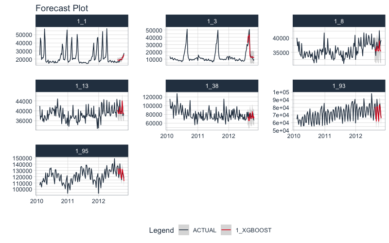
Forecast the Data
The last step we’ll cover is forecasting the test dataset. This is useful to evaluate the model using a sampling of the time series within the panel dataset. In modeltime 0.7.0, we now have modeltime_forecast(conf_by_id = TRUE) to allow the confidence intervals (prediction intervals) to be calculated by time series identifier. Note, that the modeltime_calibrate() must have been performed with an id specified.
calib_tbl %>%
    modeltime_forecast(
        new_data    = testing(splits),
        actual_data = bind_rows(training(splits), testing(splits)),
        conf_by_id  = TRUE
    ) %>%
    group_by(ID) %>%
    plot_modeltime_forecast(
        .facet_ncol  = 3,
        .interactive = FALSE
    )
Summary
We just showcased the Modeltime Workflow for Panel Data using a Global XGBOOST Model. But, this is a simple problem. And, there’s a lot more to learning time series:
- Many more algorithms
- Feature Engineering for Time Series
- Ensembling
- Machine Learning
- Deep Learning
- Scalable Modeling: 10,000+ time series
Your probably thinking how am I ever going to learn time series forecasting. Here’s the solution that will save you years of struggling.
It gets better
You’ve just scratched the surface, here’s what’s coming…
The Modeltime Ecosystem functionality is much more feature-rich than what we’ve covered here (I couldn’t possibly cover everything in this post). 😀
Here’s what I didn’t cover:
-
Feature Engineering: We can make this forecast much more accurate by including features from competition-winning strategies
-
Ensemble Modeling: We can stack models together to make super-learners that stabilize predictions.
-
Deep Learning: We can use GluonTS Deep Learning for developing high-performance, scalable forecasts.
So how are you ever going to learn time series analysis and forecasting?
You’re probably thinking:
- There’s so much to learn
- My time is precious
- I’ll never learn time series
I have good news that will put those doubts behind you.
You can learn time series analysis and forecasting in hours with my state-of-the-art time series forecasting course. 👇
High-Performance Time Series Course
Become the times series expert in your organization.
My High-Performance Time Series Forecasting in R course is available now. You’ll learn timetk and modeltime plus the most powerful time series forecasting techniques available like GluonTS Deep Learning. Become the times series domain expert in your organization.
👉 High-Performance Time Series Course.
You will learn:
- Time Series Foundations - Visualization, Preprocessing, Noise Reduction, & Anomaly Detection
- Feature Engineering using lagged variables & external regressors
- Hyperparameter Tuning - For both sequential and non-sequential models
- Time Series Cross-Validation (TSCV)
- Ensembling Multiple Machine Learning & Univariate Modeling Techniques (Competition Winner)
- Deep Learning with GluonTS (Competition Winner)
- and more.
Unlock the High-Performance Time Series Course
Have questions about Modeltime?
Make a comment in the chat below. 👇
And, if you plan on using modeltime for your business, it’s a no-brainer - Join my Time Series Course.