Tidy Discounted Cash Flow Analysis in R (for Company Valuation)
Written by Rafael Nicolas Fermin Cota
The tidy data principles are a cornerstone of financial data management and the data modeling workflow. The foundation for tidy data management is the tidyverse, a collection of R packages, that work in harmony, are built for scalability, and are taught at Business Science University. Using this infrastructure and the core tidy concepts, we can apply the tidy data principles to the Saudi Aramco Discounted Cash Flow (DCF) Valuation.
R Packages Covered
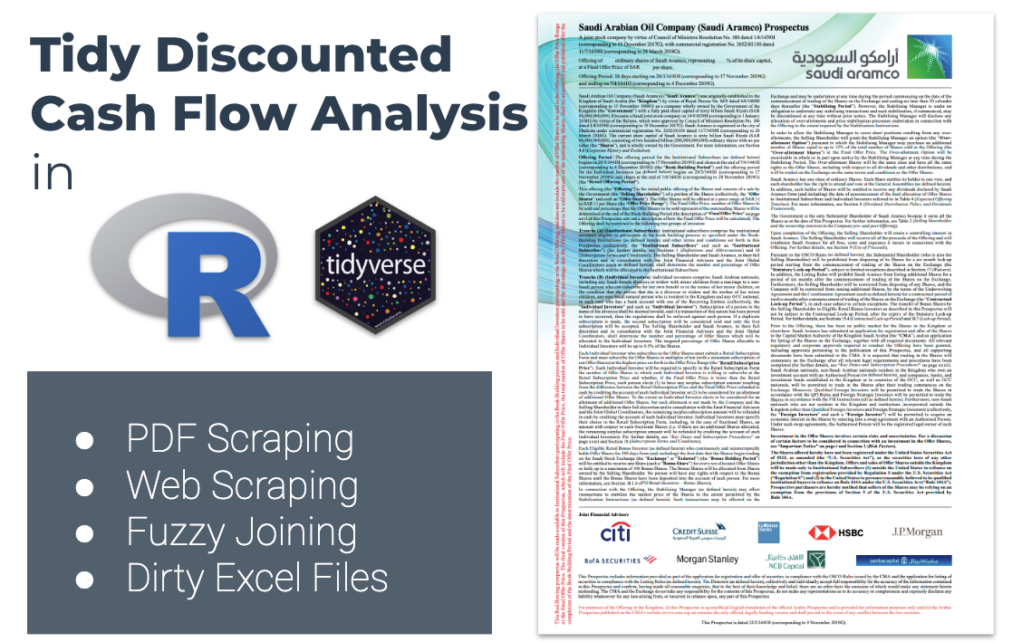
Scraping and Tidying Unclean Data
tidyverse - An ecosystem for wrangling and visualizing data in Rtabulizer - PDF Scrapingfuzzyjoin - Joining data with inexact matchingrvest - Web Scrapingtidyxl - Importing non-tabular (non-tidy) Excel Data
Tidy DCF Workflow
In this post, we’ll use the following workflow for performing and automating DCF Analysis.
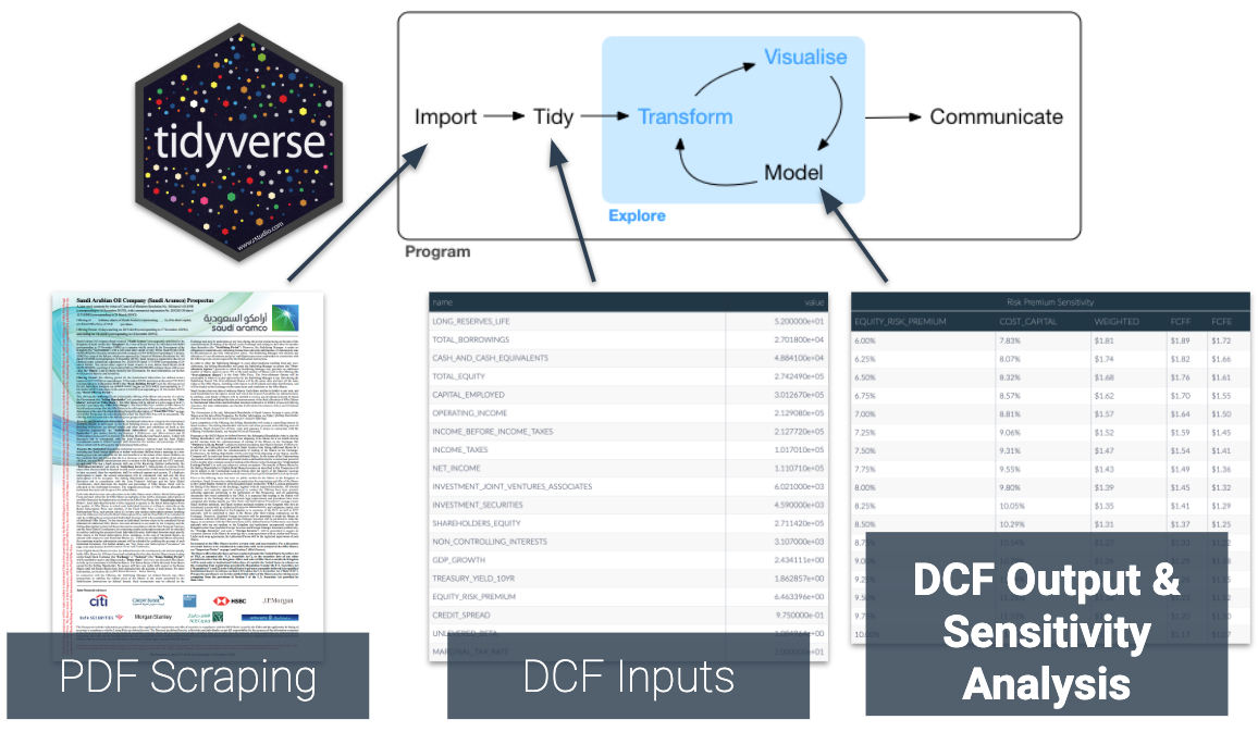
Workflow for Tidy DCF Analysis and Company Valuation
The article is split into two sections:
-
Part 1 - Data Sources: Collect DCF input data with PDF Scraping, Web Scraping, API’s, and tidy the data into a single DCF Inputs that can be used for Part 2.
-
Part 2 - DCF Company Valuation: Model Saudi Aramco’s Company Valuation. Perform sensitivity analysis given various risks to our model.
Need to learn Data Science for Business? This is an advanced tutorial, but you can get the foundational skills, advanced machine learning, business consulting, and web application development using R, Shiny (Apps), H2O (Machine Learning), AWS (Cloud), and tidyverse (Data Science). I recommend Business Science’s 4-Course R-Track for Business Bundle.
Part 1 - Data Sources
Saudi Aramco Prospectus
658 Pages of data in PDF format
Saudi Aramco has set a price range for its listing that implies the oil giant is worth between USD $1.6 trillion and US $1.7 trillion, making it potentially the world’s biggest IPO. The numbers that are laid out in the Saudi Aramco Prospectus are impressive, painting a picture of the most profitable company in the world, with almost unassailable competitive advantages. In this post, I valued Saudi Aramco between US$1.69 and US$1.83 trillion using the following R packages.
tabulizer
The tabulizer package provides a suite of tools for extracting data from PDFs. We will use the extract_tables() function to pull out tables 42 (pg 131 - gearing), 43 (pg 132 - capital), 45 (pg 133 - income statement) and 52 (pg 144 - balance sheet) from the Saudi Aramco Prospectus.
fuzzyjoin
The fuzzyjoin package is a variation on dplyr’s join operations that allows matching not just on values that match between columns, but on inexact matching. This allows the Aramco’s financial accounts (e.g., gearing, capital, income statement, balance sheet) to be quickly matched with the tables it is reported on and without having to looking for the correct location in the prospectus, a behemoth weighing in at 658 pages.
World Bank Data API
The World Bank makes available a large body of economic data from the World Development Indicators through its web API.
The WDI package for R makes it easy to search and download the annual percentage growth rate of Gross Domestic Product (GDP) for Saudi Arabia (Indicator: NY.GDP.MKTP.KD.ZG).
rvest
The rvest package makes it easy to scrape daily treasury yield curve rates from the website of the U.S. Deparment of the Treasury. Here, I use it with magrittr so that I can express complex operations as elegant pipelines composed of simple, easily understood pieces.
tidyxl
The tidyxl package imports non-tabular data from Excel files into R. It exposes cell content, position, formatting and comments in a tidy structure for further manipulation. I use tidyxl to capture Damodaran’s spreadsheets (risk premium, credit spread, unlevered beta, marginal tax rate) in a tidy fashion allowing for seamless interaction between rows and columns.
1.1 Libraries and Set Up
Install and load the following R packages to complete this tutorial. A few points to avoid frustration:
- The
tabulizer package depends on Java and rJava libraries. This can be amazingly frustrating to get set up (see my next point).
- To replicate my set up, I installed the Java 11 JDK.
- I have several versions of Java (not uncommon for developers). Using
Sys.setenv(), I pointed R to the version of Java that I wanted tabulizer to use.
Sys.setenv(JAVA_HOME="/Library/Java/JavaVirtualMachines/jdk-11.0.1.jdk/Contents/Home/")

library(knitr)
library(kableExtra)
library(ggpage)
library(magrittr)
library(tidyverse)
library(WDI)
library(pdftools)
library(tabulizer)
library(fuzzyjoin)
library(rvest)
library(janitor)
library(tidyxl)
1.2 Prospectus
In this section, I extract financial data from the prospectus, using tabulizer and fuzzyjoin. It automates work that would have taken significant manual collection and manipulation.
# Automated Data Extraction Functions for Saudi Aramco Prospectus

# Download Helper - Creates a Data folder
download.f <- function(url) {
  data.folder = file.path(getwd(), 'data')  # setup temp folder
  if (!dir.exists(data.folder)){dir.create(data.folder, F)}
  filename = file.path(data.folder, basename(url))
  if(!file.exists(filename))
    tryCatch({ download.file(url, filename, mode='wb') },
             error = function(ex) cat('', file=filename))
  message(paste0('File located at: ', filename))
  filename
}

# Tidy PDF Scraping and Fuzzy Joining Helper
extract.values.f <- function(pdf.file, page, names){
  require(tabulizer)
  require(fuzzyjoin) # regex_inner_join()

  # PDF: https://www.saudiaramco.com/-/media/images/investors/saudi-aramco-prospectus-en.pdf
  # Locate table areas
  area = case_when(
    page == 220  ~ c(459.77, 69.76, 601, 427.98), # Table 42 (pg 131)
    page == 221  ~ c(168.03, 69.76, 394.53, 404.59), # Table 43 (pg 132)
    page == 222  ~ c(180.11, 68.38, 413.04, 412.05), # Table 45 (pg 133)
    page == 233  ~ c(181.57, 70.99, 673.96, 448.91) # Table 52 (pg 144)
  )

  # Extract the tables
  extract_tables(
      pdf.file,
      pages  = page,
      area   = list(area),
      guess  = FALSE,
      output = "data.frame"
    ) %>%
    purrr::pluck(1) %>%
    map_dfc(~trimws(gsub("\\.|[[:punct:]]", "", .x))) %>%
    set_names( c("Heading", paste0("X", if(page==233){1:4}else{0:4})) ) %>%
    regex_inner_join(
      data.frame(regex_name = names, stringsAsFactors = FALSE),
      by = c(Heading = "regex_name")
    ) %>%
    select(X4) %>%
    pull() %>%
    as.numeric()
}

url <- 'https://www.saudiaramco.com/-/media/images/investors/saudi-aramco-prospectus-en.pdf'

prospectus.pdf <- download.f(url)
## File located at: /Users/nico/aramco/data/saudi-aramco-prospectus-en.pdf
For working with function programming, we solve the issue for one element, wrap the code inside a function, and then simply map extract.values.f() to a list of elements in different tables (42, 43, 45 and 52).
1.2.1 Reserves Life
Saudi Aramco’s average reserve life is 52 years, versus 17 years at it’s closest competitor, ExxonMobil. Saudi Aramco’s crude reserves are about five times (5X) that of the combined oil reserves of the five major international oil companies, comprising ExxonMobil, Shell, Chevron, Total, and BP.
# 4.6.1.2 - Long reserves life
inputs <- prospectus.pdf %>%
  pdf_text() %>%
  read_lines() %>%
  grep("proved reserves life", ., value = TRUE) %>%
  str_match_all("[0-9]+") %>%
  pluck(1) %>%
  unlist() %>%
  first() %>%
  as.numeric() %>%
  set_names(c("LONG_RESERVES_LIFE")) %>%
  as.list()

inputs %>% enframe() %>% unnest(value) %>% kable()
| name |
value |
| LONG_RESERVES_LIFE |
52 |
1.2.2 Gearing
Gearing is a measure of the degree to which Saudi Aramco’s operations are financed by debt. It is widely used by analysts and investors in the oil and gas industry to indicate a company’s financial health and flexibility.
# Table 42 - Gearing and reconciliation
inputs <- extract.values.f(
    pdf.file = prospectus.pdf,
    page     = 220,
    names    = c("Total borrowings", "Cash and cash equivalents",
                 "Total equity")
  ) %>%
  set_names(c("TOTAL_BORROWINGS", "CASH_AND_CASH_EQUIVALENTS",
              "TOTAL_EQUITY")) %>%
  as.list() %>%
  append(inputs, .)

inputs %>% enframe() %>% unnest(value) %>% kable()
| name |
value |
| LONG_RESERVES_LIFE |
52 |
| TOTAL_BORROWINGS |
27018 |
| CASH_AND_CASH_EQUIVALENTS |
48841 |
| TOTAL_EQUITY |
274249 |
1.2.3 Capital
Saudi Aramco has a comprehensive and disciplined internal approval process for capital allocation. Average capital employed is the average of Saudi Aramco’s total borrowings plus total equity at the beginning and end of the applicable period.
# Table 43 - Return on Average Capital Employed (ROACE) and reconciliation
inputs <- extract.values.f(
    pdf.file = prospectus.pdf,
    page     = 221,
    names    = c("Capital employed")
  ) %>%
  last() %>%
  set_names(c("CAPITAL_EMPLOYED")) %>%
  as.list() %>%
  append(inputs, .)

inputs %>% enframe() %>% unnest(value) %>% kable()
| name |
value |
| LONG_RESERVES_LIFE |
52 |
| TOTAL_BORROWINGS |
27018 |
| CASH_AND_CASH_EQUIVALENTS |
48841 |
| TOTAL_EQUITY |
274249 |
| CAPITAL_EMPLOYED |
301267 |
1.2.4 Income Statement
The numbers in the financial statement are impressive, painting a picture of the most profitable company in the world, with almost unassailable competitive advantages.
# Table 45 - Income statement
inputs <- extract.values.f(
    pdf.file = prospectus.pdf,
    page = 222,
    names = c("Operating income", "Income taxes",
              "Income before income taxes", "Net income")
  ) %>%
  set_names(c("OPERATING_INCOME", "INCOME_BEFORE_INCOME_TAXES",
              "INCOME_TAXES", "NET_INCOME")) %>%
  as.list() %>%
  append(inputs, .)

inputs %>% enframe() %>% unnest(value) %>% kable()
| name |
value |
| LONG_RESERVES_LIFE |
52 |
| TOTAL_BORROWINGS |
27018 |
| CASH_AND_CASH_EQUIVALENTS |
48841 |
| TOTAL_EQUITY |
274249 |
| CAPITAL_EMPLOYED |
301267 |
| OPERATING_INCOME |
212908 |
| INCOME_BEFORE_INCOME_TAXES |
212772 |
| INCOME_TAXES |
101701 |
| NET_INCOME |
111071 |
1.2.5 Balance Sheet
Saudi Aramco’s unique reserves and resources base, operational flexibility, field management, and strong cash flow generation serve as a foundation for its low gearing and flexible balance sheet.
# Table 52 - Balance sheet
inputs <- extract.values.f(
  pdf.file = prospectus.pdf,
  page     = 233,
  names    = c("Shareholders equity", "Investment in joint ventures and associates",
               "Investment in securities", "Noncontrolling interests")
  ) %>%
  purrr::discard(is.na) %>%
  set_names(c("INVESTMENT_JOINT_VENTURES_ASSOCIATES", "INVESTMENT_SECURITIES",
              "SHAREHOLDERS_EQUITY", "NON_CONTROLLING_INTERESTS")) %>%
  as.list() %>%
  append(inputs, .)

inputs %>% enframe() %>% unnest(value) %>% kable()
| name |
value |
| LONG_RESERVES_LIFE |
52 |
| TOTAL_BORROWINGS |
27018 |
| CASH_AND_CASH_EQUIVALENTS |
48841 |
| TOTAL_EQUITY |
274249 |
| CAPITAL_EMPLOYED |
301267 |
| OPERATING_INCOME |
212908 |
| INCOME_BEFORE_INCOME_TAXES |
212772 |
| INCOME_TAXES |
101701 |
| NET_INCOME |
111071 |
| INVESTMENT_JOINT_VENTURES_ASSOCIATES |
6021 |
| INVESTMENT_SECURITIES |
4590 |
| SHAREHOLDERS_EQUITY |
271142 |
| NON_CONTROLLING_INTERESTS |
3107 |
1.3 World Bank GDP
For Saudi Aramco, the growth rate in earnings corresponds closely to the growth in Saudi Arabia’s GDP. The reason is simple. Saudi Arabia derives almost 80% of its GDP from oil.
# World Development Indicators (WDI)
inputs <- WDI::WDI(
    country=c("SAU"),
    indicator="NY.GDP.MKTP.KD.ZG", # = GDP growth (annual %)
    start=2018,
    end=2018
  ) %>%
  pull("NY.GDP.MKTP.KD.ZG") %>%
  set_names(c("GDP_GROWTH")) %>% #  (annual %)
  as.list() %>%
  append(inputs, .)

inputs %>% enframe() %>% unnest(value) %>% kable()
| name |
value |
| LONG_RESERVES_LIFE |
5.200000e+01 |
| TOTAL_BORROWINGS |
2.701800e+04 |
| CASH_AND_CASH_EQUIVALENTS |
4.884100e+04 |
| TOTAL_EQUITY |
2.742490e+05 |
| CAPITAL_EMPLOYED |
3.012670e+05 |
| OPERATING_INCOME |
2.129080e+05 |
| INCOME_BEFORE_INCOME_TAXES |
2.127720e+05 |
| INCOME_TAXES |
1.017010e+05 |
| NET_INCOME |
1.110710e+05 |
| INVESTMENT_JOINT_VENTURES_ASSOCIATES |
6.021000e+03 |
| INVESTMENT_SECURITIES |
4.590000e+03 |
| SHAREHOLDERS_EQUITY |
2.711420e+05 |
| NON_CONTROLLING_INTERESTS |
3.107000e+03 |
| GDP_GROWTH |
2.434111e+00 |
1.4 U.S.Treasuries
We use the 10-Year U.S. Treasury Rate because the currency choice for the Saudi Aramco discounted cash flow valuation is U.S. dollars.
treasury.rates.f <- function(year=2019){
  require(rvest)
  require(janitor)
  # year=calendar year to pull results for

  # Data is generally updated at the end of each business day
  rate_url <- paste(
    'https://www.treasury.gov/resource-center/data-chart-center/interest-rates/Pages/TextView.aspx?data=yieldYear&year=',
    year,
    sep=''
  )

  #  1 mo, 2 mo, 3 mo, 6 mo, 1 yr, 2 yr, 3 yr, 5 yr, 7 yr, 10 yr, 20 yr, 30 yr
  rates_raw <- read_html(rate_url) %>%
    html_node('.t-chart') %>%
    html_table()

  # Returns treasury rates for the given duration
  rates <- rates_raw %>%
    clean_names(.) %>%
    mutate(
      date = as.Date(date, "%m/%d/%y"),
      month = factor(months(date), levels=month.name)
    ) %>%
    mutate_at(
      vars(-one_of("date", "month")),
      as.numeric
    )

  summary <- rates %>%
    select(-date) %>%
    group_by(month) %>%
    summarise_all(list(mean))

  return(summary)
}

rates <- treasury.rates.f(2019) # last update dec 7, 2019

inputs <- rates %>%
  select(x10_yr) %>%
  slice(n()) %>% # Dec 10_yr Avg.
  pull() %>%
  set_names(c("TREASURY_YIELD_10YR")) %>%
  as.list() %>%
  append(inputs, .)

inputs %>% enframe() %>% unnest(value) %>% kable()
| name |
value |
| LONG_RESERVES_LIFE |
5.200000e+01 |
| TOTAL_BORROWINGS |
2.701800e+04 |
| CASH_AND_CASH_EQUIVALENTS |
4.884100e+04 |
| TOTAL_EQUITY |
2.742490e+05 |
| CAPITAL_EMPLOYED |
3.012670e+05 |
| OPERATING_INCOME |
2.129080e+05 |
| INCOME_BEFORE_INCOME_TAXES |
2.127720e+05 |
| INCOME_TAXES |
1.017010e+05 |
| NET_INCOME |
1.110710e+05 |
| INVESTMENT_JOINT_VENTURES_ASSOCIATES |
6.021000e+03 |
| INVESTMENT_SECURITIES |
4.590000e+03 |
| SHAREHOLDERS_EQUITY |
2.711420e+05 |
| NON_CONTROLLING_INTERESTS |
3.107000e+03 |
| GDP_GROWTH |
2.434111e+00 |
| TREASURY_YIELD_10YR |
1.862857e+00 |
1.5 Damodaran Online
1.5.1 Risk Premium
Damodaran’s equity risk premium is calculated by adding the mature market premium estimated for the US to the country-specific risk premium. To arrive at Saudi Arabia’s equity risk premium, Damodaran augmented the default spread by a scaling factor to reflect the higher risk of equity.
risk.premium.f <- function(){
  require(tidyxl)

  url <- 'http://pages.stern.nyu.edu/~adamodar/pc/datasets/ctrypremJuly19.xlsx'
  data_file <- download.f(url)
  tidy_table <- xlsx_cells(data_file, sheets = "ERPs by country") %>%
    filter(!is_blank, row >= 7 & row <=162) %>%
    select(row, col, data_type, character, numeric)
  # equity risk premium with a country risk premium for Saudi Arabia added to
  # the mature market premium estimated for the US.
  i <- tidy_table %>% filter(character=="Saudi Arabia") %>% pull(row)
  j <- tidy_table %>% filter(character=="Total Equity Risk Premium") %>% pull(col)
  v <- tidy_table %>% filter(row == i & col == j) %>% pull(numeric)
  return(v * 100)
}

erp <- risk.premium.f()
## File located at: /Users/nico/aramco/data/ctrypremJuly19.xlsx
inputs <- erp %>%
  set_names(c("EQUITY_RISK_PREMIUM")) %>%
  as.list() %>%
  append(inputs, .)

inputs %>% enframe() %>% unnest(value) %>% kable()
| name |
value |
| LONG_RESERVES_LIFE |
5.200000e+01 |
| TOTAL_BORROWINGS |
2.701800e+04 |
| CASH_AND_CASH_EQUIVALENTS |
4.884100e+04 |
| TOTAL_EQUITY |
2.742490e+05 |
| CAPITAL_EMPLOYED |
3.012670e+05 |
| OPERATING_INCOME |
2.129080e+05 |
| INCOME_BEFORE_INCOME_TAXES |
2.127720e+05 |
| INCOME_TAXES |
1.017010e+05 |
| NET_INCOME |
1.110710e+05 |
| INVESTMENT_JOINT_VENTURES_ASSOCIATES |
6.021000e+03 |
| INVESTMENT_SECURITIES |
4.590000e+03 |
| SHAREHOLDERS_EQUITY |
2.711420e+05 |
| NON_CONTROLLING_INTERESTS |
3.107000e+03 |
| GDP_GROWTH |
2.434111e+00 |
| TREASURY_YIELD_10YR |
1.862857e+00 |
| EQUITY_RISK_PREMIUM |
6.463396e+00 |
1.5.2 Credit Spread
We use a credit spread that lenders would charge a large integrated oil & gas company with a specific credit rating, and add it to the avg. 10 year U.S. treasury rate to arrive at Saudi Aramco’s cost of debt.
rating.spread.f <- function(){
  require(readxl)

  # Ratings, Interest Coverage Ratios and Default Spread
  url <- 'http://www.stern.nyu.edu/~adamodar/pc/ratings.xls'
  data_file <- download.f(url)
  v <- read_excel(
    data_file, sheet = "Start here Ratings sheet",
    range = "A18:D33") %>% # A18:D33 -> rating table for large manufacturing firms
    janitor::clean_names() %>%
    filter(rating_is=="A1/A+") %>%
    pull(spread_is)
  return(v * 100)
}

cs <- rating.spread.f()
## File located at: /Users/nico/aramco/data/ratings.xls
inputs <- cs %>%
  set_names(c("CREDIT_SPREAD")) %>%
  as.list() %>%
  append(inputs, .)

inputs %>% enframe() %>% unnest(value) %>% kable()
| name |
value |
| LONG_RESERVES_LIFE |
5.200000e+01 |
| TOTAL_BORROWINGS |
2.701800e+04 |
| CASH_AND_CASH_EQUIVALENTS |
4.884100e+04 |
| TOTAL_EQUITY |
2.742490e+05 |
| CAPITAL_EMPLOYED |
3.012670e+05 |
| OPERATING_INCOME |
2.129080e+05 |
| INCOME_BEFORE_INCOME_TAXES |
2.127720e+05 |
| INCOME_TAXES |
1.017010e+05 |
| NET_INCOME |
1.110710e+05 |
| INVESTMENT_JOINT_VENTURES_ASSOCIATES |
6.021000e+03 |
| INVESTMENT_SECURITIES |
4.590000e+03 |
| SHAREHOLDERS_EQUITY |
2.711420e+05 |
| NON_CONTROLLING_INTERESTS |
3.107000e+03 |
| GDP_GROWTH |
2.434111e+00 |
| TREASURY_YIELD_10YR |
1.862857e+00 |
| EQUITY_RISK_PREMIUM |
6.463396e+00 |
| CREDIT_SPREAD |
9.750000e-01 |
1.5.3 Unlevered Beta
In calculating the cost of equity, we use an unlevered beta for Saudi Aramco based on integrated oil companies for both cash flow models: (1) cash flows after reinvestment needs and taxes, but before debt payments (FCFF); and (2) cash flows after taxes, reinvestments, and debt payments (FCFE).
# Effective Tax rate, Unlevered beta
unlevered.beta.f <- function(){
  require(readxl)

  # Unlevered Betas (Global)
  url <- 'http://www.stern.nyu.edu/~adamodar/pc/datasets/betaGlobal.xls'
  data_file <- download.f(url)

  v <- read_excel(data_file, sheet = "Industry Averages", range = "A10:F106") %>%
    janitor::clean_names() %>%
    filter(industry_name=="Oil/Gas (Integrated)") %>%
    pull(unlevered_beta)
  return(v)
}

ub <- unlevered.beta.f()
## File located at: /Users/nico/aramco/data/betaGlobal.xls
inputs <- ub %>%
  set_names(c("UNLEVERED_BETA")) %>%
  as.list %>%
  append(inputs, .)

inputs %>% enframe() %>% unnest(value) %>% kable()
| name |
value |
| LONG_RESERVES_LIFE |
5.200000e+01 |
| TOTAL_BORROWINGS |
2.701800e+04 |
| CASH_AND_CASH_EQUIVALENTS |
4.884100e+04 |
| TOTAL_EQUITY |
2.742490e+05 |
| CAPITAL_EMPLOYED |
3.012670e+05 |
| OPERATING_INCOME |
2.129080e+05 |
| INCOME_BEFORE_INCOME_TAXES |
2.127720e+05 |
| INCOME_TAXES |
1.017010e+05 |
| NET_INCOME |
1.110710e+05 |
| INVESTMENT_JOINT_VENTURES_ASSOCIATES |
6.021000e+03 |
| INVESTMENT_SECURITIES |
4.590000e+03 |
| SHAREHOLDERS_EQUITY |
2.711420e+05 |
| NON_CONTROLLING_INTERESTS |
3.107000e+03 |
| GDP_GROWTH |
2.434111e+00 |
| TREASURY_YIELD_10YR |
1.862857e+00 |
| EQUITY_RISK_PREMIUM |
6.463396e+00 |
| CREDIT_SPREAD |
9.750000e-01 |
| UNLEVERED_BETA |
1.084964e+00 |
1.5.4 Marginal Tax
The marginal tax rate is the number we use to compute Saudi Aramco’s after-tax cost of debt. Given Saudi Aramco’s marginal corporate tax rate, the after-tax cost of debt equates to the treasury rate plus the credit spread that lenders would charge Saudi Aramco multiplied by one minus the marginal tax rate.
marginal.tax.f <- function(){
  require(readxl)
  # data_file <- file.path("data", "countrytaxrates.xls")
  url <- 'http://www.stern.nyu.edu/~adamodar/pc/datasets/countrytaxrates.xls'
  data_file <- download.f(url)
  # Corporate Marginal Tax Rates - By country
  v <- read_excel(data_file, sheet = "Sheet1") %>%
    janitor::clean_names() %>%
    filter(country=="Saudi Arabia") %>%
    pull(x2018)
  return(v * 100)
}

mtr <- marginal.tax.f()
## File located at: /Users/nico/aramco/data/countrytaxrates.xls
inputs <- mtr %>%
  set_names(c("MARGINAL_TAX_RATE")) %>%
  as.list %>%
  append(inputs, .)

inputs %>% enframe() %>% unnest(value) %>% kable()
| name |
value |
| LONG_RESERVES_LIFE |
5.200000e+01 |
| TOTAL_BORROWINGS |
2.701800e+04 |
| CASH_AND_CASH_EQUIVALENTS |
4.884100e+04 |
| TOTAL_EQUITY |
2.742490e+05 |
| CAPITAL_EMPLOYED |
3.012670e+05 |
| OPERATING_INCOME |
2.129080e+05 |
| INCOME_BEFORE_INCOME_TAXES |
2.127720e+05 |
| INCOME_TAXES |
1.017010e+05 |
| NET_INCOME |
1.110710e+05 |
| INVESTMENT_JOINT_VENTURES_ASSOCIATES |
6.021000e+03 |
| INVESTMENT_SECURITIES |
4.590000e+03 |
| SHAREHOLDERS_EQUITY |
2.711420e+05 |
| NON_CONTROLLING_INTERESTS |
3.107000e+03 |
| GDP_GROWTH |
2.434111e+00 |
| TREASURY_YIELD_10YR |
1.862857e+00 |
| EQUITY_RISK_PREMIUM |
6.463396e+00 |
| CREDIT_SPREAD |
9.750000e-01 |
| UNLEVERED_BETA |
1.084964e+00 |
| MARGINAL_TAX_RATE |
2.000000e+01 |
Part 2 - DCF Company Valuation
We now have all of the data needed to calculate the Company Valuation.
- Calculate the discount rate or rates to use in the valuation for Saudi Aramco.
- cost of equity for equity investors (FCFE)
- cost of capital for all claimholders (FCFF)
-
Calculate the current earnings and cash flows of Saudi Aramco for equity investors and for all claimholders.
-
Calculate the future earnings and cash flows of Saudi Aramco by estimating an expected growth rate in earnings (GDP growth).
- Calculate Saudi Aramco’s Discounted Cash Flow valuations.
equity.valuation.f <- function(inp){

  for (j in 1:length(inp)) assign(names(inp)[j], inp[[j]])
  #-------------------------------------------------------------------------------------
  # Calculated inputs

  EFFECTIVE_TAX_RATE <- INCOME_TAXES / INCOME_BEFORE_INCOME_TAXES
  INVESTED_CAPITAL <- CAPITAL_EMPLOYED - CASH_AND_CASH_EQUIVALENTS
  DEBT_RATIO <- TOTAL_BORROWINGS / ( TOTAL_BORROWINGS + TOTAL_EQUITY )

  COST_DEBT <- ( CREDIT_SPREAD + TREASURY_YIELD_10YR ) / 100
  COST_EQUITY <- ( TREASURY_YIELD_10YR + UNLEVERED_BETA * EQUITY_RISK_PREMIUM ) / 100
  COST_CAPITAL <- COST_DEBT * ( 1 - ( MARGINAL_TAX_RATE / 100 ) ) * DEBT_RATIO +
    COST_EQUITY * ( 1 - DEBT_RATIO )

  NUMBER_YEARS <- LONG_RESERVES_LIFE

  #-------------------------------------------------------------------------------------
  # Free Cash Flow to Equity (FCFE)

  EXPECTED_RETURN_EQUITY <- NET_INCOME / SHAREHOLDERS_EQUITY
  EXPECTED_GROWTH_EARNINGS <- GDP_GROWTH / 100
  PAYOUT_RATIO <- 1 - EXPECTED_GROWTH_EARNINGS / EXPECTED_RETURN_EQUITY

  VALUE_EQUITY <- NET_INCOME * PAYOUT_RATIO *
    ( 1 - ( ( 1 + EXPECTED_GROWTH_EARNINGS ) ^ NUMBER_YEARS /
              ( 1 + COST_EQUITY ) ^ NUMBER_YEARS ) ) /
    ( COST_EQUITY - EXPECTED_GROWTH_EARNINGS )

  FCFE_EQUITY_VALUATION <- VALUE_EQUITY + CASH_AND_CASH_EQUIVALENTS +
    INVESTMENT_JOINT_VENTURES_ASSOCIATES + INVESTMENT_SECURITIES

  #-------------------------------------------------------------------------------------
  # Free Cash Flow to Firm (FCFF)
  EXPECTED_GROWTH_RATE <- GDP_GROWTH / 100
  EXPECTED_ROIC <- OPERATING_INCOME * ( 1 - EFFECTIVE_TAX_RATE ) / INVESTED_CAPITAL
  REINVESTMENT_RATE <- EXPECTED_GROWTH_RATE / EXPECTED_ROIC

  EXPECTED_OPERATING_INCOME_AFTER_TAX <- OPERATING_INCOME *
    ( 1 - EFFECTIVE_TAX_RATE ) * ( 1 + EXPECTED_GROWTH_RATE )

  EXPECTED_FCFF <- EXPECTED_OPERATING_INCOME_AFTER_TAX * ( 1 - REINVESTMENT_RATE )

  VALUE_OPERATING_ASSETS <- EXPECTED_FCFF *
    ( 1 - ( ( 1 + EXPECTED_GROWTH_RATE ) ^ NUMBER_YEARS /
              ( 1 + COST_CAPITAL ) ^ NUMBER_YEARS ) ) /
    ( COST_CAPITAL - EXPECTED_GROWTH_RATE )

  FCFF_EQUITY_VALUATION <- VALUE_OPERATING_ASSETS + CASH_AND_CASH_EQUIVALENTS +
    INVESTMENT_JOINT_VENTURES_ASSOCIATES + INVESTMENT_SECURITIES -
    TOTAL_BORROWINGS - NON_CONTROLLING_INTERESTS

  #-------------------------------------------------------------------------------------
  # Use set_names to name the elements of the vector
  out <- c(INVESTED_CAPITAL, DEBT_RATIO, EFFECTIVE_TAX_RATE) %>%
    set_names(c("INVESTED_CAPITAL", "DEBT_RATIO", "EFFECTIVE_TAX_RATE"))

  out <- c(NUMBER_YEARS, COST_CAPITAL, COST_EQUITY, COST_DEBT) %>%
    set_names(c("NUMBER_YEARS", "COST_CAPITAL", "COST_EQUITY", "COST_DEBT")) %>%
    as.list %>% append(out)

  out <- c(FCFE_EQUITY_VALUATION, VALUE_EQUITY, PAYOUT_RATIO,
           EXPECTED_GROWTH_EARNINGS, EXPECTED_RETURN_EQUITY) %>%
    set_names(c("FCFE_EQUITY_VALUATION", "VALUE_EQUITY", "PAYOUT_RATIO",
                "EXPECTED_GROWTH_EARNINGS", "EXPECTED_RETURN_EQUITY")) %>%
    as.list %>% append(out)

  out <- c(FCFF_EQUITY_VALUATION, VALUE_OPERATING_ASSETS, EXPECTED_FCFF,
           EXPECTED_OPERATING_INCOME_AFTER_TAX, REINVESTMENT_RATE,
           EXPECTED_ROIC, EXPECTED_GROWTH_RATE) %>%
    set_names(c("FCFF_EQUITY_VALUATION", "VALUE_OPERATING_ASSETS", "EXPECTED_FCFF",
                "EXPECTED_OPERATING_INCOME_AFTER_TAX", "REINVESTMENT_RATE",
                "EXPECTED_ROIC", "EXPECTED_GROWTH_RATE")) %>%
    as.list %>% append(out)
  #-------------------------------------------------------------------------------------

  return(out)
}

output <- equity.valuation.f(inputs)

output %>% enframe() %>% unnest(value) %>% kable()
| name |
value |
| FCFF_EQUITY_VALUATION |
1.765728e+06 |
| VALUE_OPERATING_ASSETS |
1.736401e+06 |
| EXPECTED_FCFF |
1.075534e+05 |
| EXPECTED_OPERATING_INCOME_AFTER_TAX |
1.138473e+05 |
| REINVESTMENT_RATE |
5.528360e-02 |
| EXPECTED_ROIC |
4.402954e-01 |
| EXPECTED_GROWTH_RATE |
2.434110e-02 |
| FCFE_EQUITY_VALUATION |
1.613303e+06 |
| VALUE_EQUITY |
1.553851e+06 |
| PAYOUT_RATIO |
9.405795e-01 |
| EXPECTED_GROWTH_EARNINGS |
2.434110e-02 |
| EXPECTED_RETURN_EQUITY |
4.096414e-01 |
| NUMBER_YEARS |
5.200000e+01 |
| COST_CAPITAL |
8.283050e-02 |
| COST_EQUITY |
8.875410e-02 |
| COST_DEBT |
2.837860e-02 |
| INVESTED_CAPITAL |
2.524260e+05 |
| DEBT_RATIO |
8.968120e-02 |
| EFFECTIVE_TAX_RATE |
4.779811e-01 |
2.1 DCF Summary
Below, I valued Saudi Aramco at about USD$1.76 trillion using a weighted DCF equity valuation:
- 50% for Operating income & FCFF
- 50% for Equity income & FCFE.
tibble(
    Weighted = 0.5 * (output$FCFF_EQUITY_VALUATION + output$FCFE_EQUITY_VALUATION) / 1000000,
    FCFF     = output$FCFF_EQUITY_VALUATION / 1000000,
    FCFE     = output$FCFE_EQUITY_VALUATION / 1000000
  ) %>%
  mutate_all(scales::dollar) %>%
  kable() %>%
  kable_styling(c("striped", "bordered")) %>%
  add_header_above(c("Saudi Aramco Equity Valuation ($ trillions)" = 3))
Saudi Aramco Equity Valuation ($ trillions) |
|---|
| Weighted |
FCFF |
FCFE |
| $1.69 |
$1.77 |
$1.61 |
2.2 Sensitivity
It is very likely that investors will reward Saudi Aramco for:
- Ultralong reserve life
- Lower gearing than each of the five major international oil companies
- Ability to execute some of the world’s largest upstream and downstream capital projects
- Higher operating cash flow, free cash flow, EBIT, EBITDA, and Return on Average Capital Employed (ROACE) than each of the five major international oil companies
However, investors could also penalize Saudi Aramco for the geopolitical risk and the central banking conspiracy to keep interest rates low.
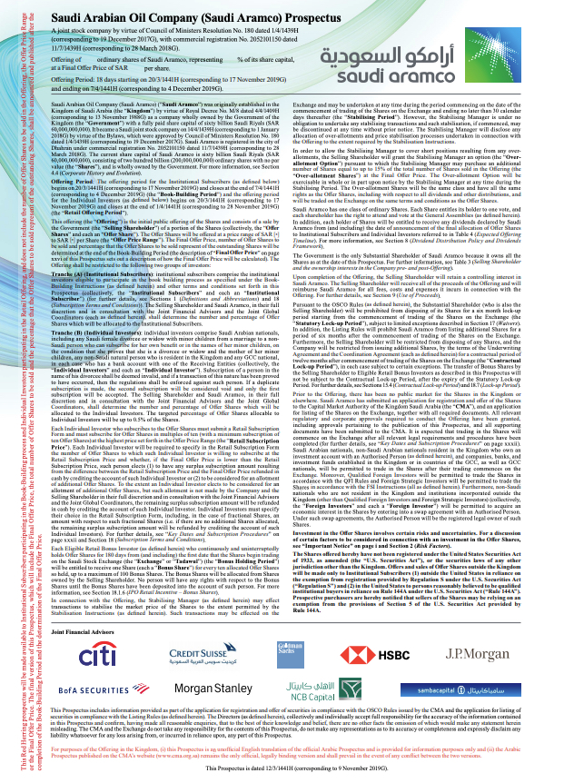
2.2.1 Risk Premium Sensitivity
Given the risk of attacks against Saudi Aramco’ oil and gas infrastructure, there is a chance that the equity risk premium and the cost of capital could go up. However, if we remove that geopolitical risk from consideration and look at the remaining risk, Aramco is a remarkably safe investment, with the mind-boggling profits and cash flows and access to huge oil reserves consisting of $201.4$ billion barrels of crude oil and condensate, $25.4$ billion barrels of NGLs, and $185.7$ trillion standard cubic feet of natural gas.
# Equity Risk Premium
out <- map(
  seq(6, 10, 0.25),
  ~list_modify(
    inputs,
    EQUITY_RISK_PREMIUM=.x
  ) %>%
    equity.valuation.f(.)
)

map2_dfr(
    out,
    seq(6, 10, 0.25),
    ~list(
      EQUITY_RISK_PREMIUM=.y,
      COST_CAPITAL=.x$COST_CAPITAL*100,
      WEIGHTED=(.x$FCFF_EQUITY_VALUATION+.x$FCFE_EQUITY_VALUATION) / 2 / 1000000,
      FCFF=.x$FCFF_EQUITY_VALUATION / 1000000,
      FCFE=.x$FCFE_EQUITY_VALUATION / 1000000
    )
  ) %>%
  mutate_at(
    vars(one_of("FCFF", "FCFE", "WEIGHTED")),
    scales::dollar
  ) %>%
  mutate_at(
    vars(one_of("EQUITY_RISK_PREMIUM", "COST_CAPITAL")),
    function(v) sprintf(v, fmt = "%.2f%%")
  ) %>%
  kable() %>%
  add_header_above(c("Risk Premium Sensitivity" = 5))
Risk Premium Sensitivity |
|---|
| EQUITY_RISK_PREMIUM |
COST_CAPITAL |
WEIGHTED |
FCFF |
FCFE |
| 6.00% |
7.83% |
$1.81 |
$1.89 |
$1.72 |
| 6.25% |
8.07% |
$1.74 |
$1.82 |
$1.66 |
| 6.50% |
8.32% |
$1.68 |
$1.76 |
$1.61 |
| 6.75% |
8.57% |
$1.62 |
$1.70 |
$1.55 |
| 7.00% |
8.81% |
$1.57 |
$1.64 |
$1.50 |
| 7.25% |
9.06% |
$1.52 |
$1.59 |
$1.45 |
| 7.50% |
9.31% |
$1.47 |
$1.54 |
$1.41 |
| 7.75% |
9.55% |
$1.43 |
$1.49 |
$1.36 |
| 8.00% |
9.80% |
$1.39 |
$1.45 |
$1.32 |
| 8.25% |
10.05% |
$1.35 |
$1.41 |
$1.29 |
| 8.50% |
10.29% |
$1.31 |
$1.37 |
$1.25 |
| 8.75% |
10.54% |
$1.27 |
$1.33 |
$1.22 |
| 9.00% |
10.79% |
$1.24 |
$1.29 |
$1.18 |
| 9.25% |
11.04% |
$1.21 |
$1.26 |
$1.15 |
| 9.50% |
11.28% |
$1.18 |
$1.23 |
$1.12 |
| 9.75% |
11.53% |
$1.15 |
$1.20 |
$1.10 |
| 10.00% |
11.78% |
$1.12 |
$1.17 |
$1.07 |
2.2.2 Treasury Yield Sensitivity
Central banks around the world have conspired to keep interest rates low and artificially push up the price of financial assets. The end game in this story is that the central banks will eventually be forced to face reality, where the U.S. 10-Year Treasury will rise to normal levels and the value of Saudi Aramco could decrease.
out <- map(
  seq(1, 4, 0.25),
  ~list_modify(
    inputs,
    TREASURY_YIELD_10YR=.x
  ) %>%
    equity.valuation.f(.)
)

map2_dfr(
    out,
    seq(1, 4, 0.25),
    ~list(
      TREASURY_YIELD_10YR = .y,
      WEIGHTED = (.x$FCFF_EQUITY_VALUATION+.x$FCFE_EQUITY_VALUATION) / 2 / 1000000,
      FCFF = .x$FCFF_EQUITY_VALUATION / 1000000,
      FCFE = .x$FCFE_EQUITY_VALUATION / 1000000
    )
  ) %>%
  # arrange(-TREASURY_YIELD_10YR) %>%
  mutate_at(
    vars(one_of("FCFF", "FCFE", "WEIGHTED")),
    scales::dollar
  ) %>%
  mutate_at(
    vars(one_of("TREASURY_YIELD_10YR")),
    function(v) sprintf(v, fmt = "%.2f%%")
  ) %>%
  kable() %>%
  add_header_above(c("Treasury Yield Sensitivity" = 4))
Treasury Yield Sensitivity |
|---|
| TREASURY_YIELD_10YR |
WEIGHTED |
FCFF |
FCFE |
| 1.00% |
$1.91 |
$2.00 |
$1.81 |
| 1.25% |
$1.84 |
$1.93 |
$1.75 |
| 1.50% |
$1.78 |
$1.86 |
$1.69 |
| 1.75% |
$1.72 |
$1.79 |
$1.64 |
| 2.00% |
$1.66 |
$1.73 |
$1.59 |
| 2.25% |
$1.61 |
$1.68 |
$1.54 |
| 2.50% |
$1.56 |
$1.62 |
$1.49 |
| 2.75% |
$1.51 |
$1.57 |
$1.45 |
| 3.00% |
$1.46 |
$1.52 |
$1.40 |
| 3.25% |
$1.42 |
$1.48 |
$1.36 |
| 3.50% |
$1.38 |
$1.43 |
$1.33 |
| 3.75% |
$1.34 |
$1.39 |
$1.29 |
| 4.00% |
$1.31 |
$1.35 |
$1.26 |
2.2.3 Reserves Life Sensitivity
Saudi Aramco’s oil equivalent reserves were sufficient for proved reserves life of $52$ years, which was significantly longer than the $9$ to $17$ year proved reserves life of any of the five major international oil companies based on publicly available information.
out <- map(
  40:52, # Long reserves life
  ~list_modify(
    inputs,
    LONG_RESERVES_LIFE=.x
  ) %>%
    equity.valuation.f(.)
)

map_dfr(
    out,
    ~list(
      RESERVES_LIFE = .x$NUMBER_YEARS,
      WEIGHTED      = (.x$FCFF_EQUITY_VALUATION+.x$FCFE_EQUITY_VALUATION) / 2 / 1000000,
      FCFF = .x$FCFF_EQUITY_VALUATION / 1000000,
      FCFE = .x$FCFE_EQUITY_VALUATION / 1000000
    )
  ) %>%
  arrange(-RESERVES_LIFE) %>%
  mutate_at(
    vars(one_of("FCFF", "FCFE", "WEIGHTED")),
    scales::dollar
  ) %>%
  kable() %>%
  add_header_above(c("Reserves Life Sensitivity" = 4))
Reserves Life Sensitivity |
|---|
| RESERVES_LIFE |
WEIGHTED |
FCFF |
FCFE |
| 52 |
$1.69 |
$1.77 |
$1.61 |
| 51 |
$1.68 |
$1.76 |
$1.61 |
| 50 |
$1.68 |
$1.75 |
$1.60 |
| 49 |
$1.67 |
$1.75 |
$1.60 |
| 48 |
$1.67 |
$1.74 |
$1.59 |
| 47 |
$1.66 |
$1.73 |
$1.59 |
| 46 |
$1.65 |
$1.73 |
$1.58 |
| 45 |
$1.65 |
$1.72 |
$1.58 |
| 44 |
$1.64 |
$1.71 |
$1.57 |
| 43 |
$1.63 |
$1.70 |
$1.56 |
| 42 |
$1.62 |
$1.69 |
$1.56 |
| 41 |
$1.61 |
$1.68 |
$1.55 |
| 40 |
$1.60 |
$1.67 |
$1.54 |
Conclusion
We performed a Saudi Aramco Discounted Cash Flow (DCF) Valuation leveraging:
tidyverse - An ecosystem for wrangling and visualizing data in Rtabulizer - PDF Scrapingfuzzyjoin - Joining data with inexact matchingrvest - Web Scrapingtidyxl - Importing non-tabular (non-tidy) Excel Data
If you would like to learn these skills, I recommend Business Science University’s 4-Course R-Track Program. This program teaches you the essential skills to apply data science to finance and accelerate you career. Learn more.
About the Author
Business Science would like to thank the author, Rafael Nicolas Fermin Cota (Follow Nico here), for contributing this powerful article on “Tidy Discounted Cash Flow Valuation”.
Rafael Nicolas Fermin Cota (Nico) founded and is the CEO at 162 Labs. He is also a part-time faculty member at the National University of Singapore.
Prior to founding 162 Labs, Nico co-founded and led the technology and research teams at OneSixtyTwo Capital. In this role, he was responsible for quantitative application development supporting various systematic trading strategies and the integration of trading/market data-driven technologies.