Tidy Time Series Forecasting in R with Spark
Written by Matt Dancho
I’m SUPER EXCITED to show fellow time-series enthusiasts a new way that we can scale time series analysis using an amazing technology called Spark!
Without Spark, large-scale forecasting projects of 10,000 time series can take days to run because of long-running for-loops and the need to test many models on each time series.
Spark has been widely accepted as a “big data” solution, and we’ll use it to scale-out (distribute) our time series analysis to Spark Clusters, and run our analysis in parallel.
TLDR
-
Spark is an amazing technology for processing large-scale data science workloads.
-
Modeltime is a state-of-the-art forecasting library that I personally developed for “Tidy Forecasting” in R. Modeltime now integrates a Spark Backend with capability of forecasting 10,000+ time series using distributed Spark Clusters.
-
I show an introductory tutorial to get you started. Readers can sign up for a Free Live Training using Modeltime and Spark where we’ll cover more detail that we couldn’t cover during this introductory tutorial including:
- Forecasting Ensembles (New Capability)
- More Advanced Time Series Algorithms
- Feature Engineering at Scale
- Special Offers on Courses
Free Training: 3-Tips to Scale Forecasting
As mentioned above, we are hosting a Free Training: 3-Tips to Scale Forecasting. This will be a 1-hour full-code training with 3 tips to scale your forecasting.
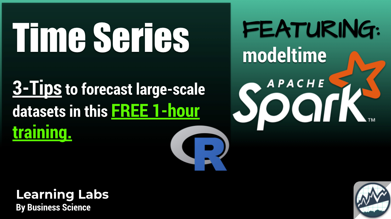
Click image for Free Time Series Training
Register Here for Free Training
What is Spark?
I feel like I’ve unlocked infinite power.
If you’re like me, you have heard this term, “Spark”, but maybe you haven’t tried it yet. That was me about 2-months ago… Boy, am I glad I tried it. I feel like I’ve unlocked infinite power.
Spark’s Best Qualities
According to Spark’s website, Spark is a “unified analytics engine for large-scale data processing.”

This means that Spark has the following amazing qualities:
-
Spark is Unified: We can use different languages like Python, R, SQL and Java to interact with Spark.
-
Spark is made for Large-Scale: We can run workloads 100X faster versus Hadoop (according to Spark).
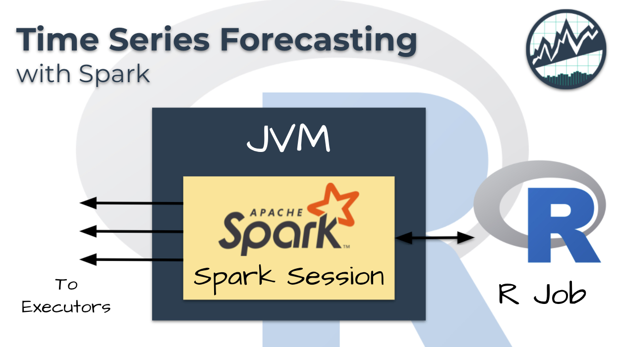
How Spark Works
Here’s a picture showing how Spark works.
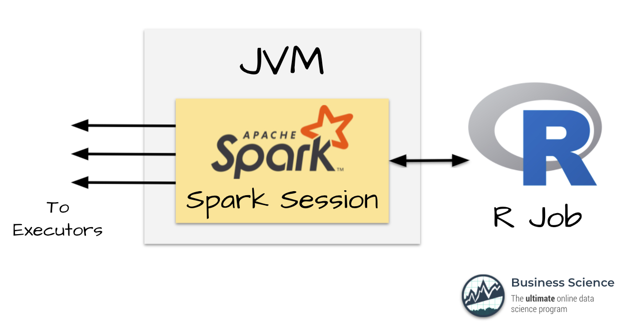
How Spark Works
-
Spark runs on Java Virtual Machines (JVMs), which allow Spark to run and distribute workloads very fast.
-
But most of us aren’t Java Programmers (we’re R and Python programmers), so Spark has an interface to R and Python.
-
This means we can communicate with Spark via R, and send the work to Spark Executors all from the comfort of R. Boom. 💥
What is Modeltime?
Modeltime is a time series forecasting framework for “tidy time series forecasting”.
Tidy Modeling
Tidymodels is like Scikit Learn, but better.
The “Tidy” in “Tidy time series forecasting” is because modeltime builds on top of tidymodels, a collection of packages for modeling and machine learning using tidyverse principles.
I equate Tidymodels in R to Scikit Learn in Python… Tidymodels is like Scikit Learn, but better. It’s simply easier to use especially when it comes to feature engineering (very important for time series), and I become more productive because of it.
tidymodels.org
Tidy Time Series Forecasting
Because modeltime builds on top of Tidymodels, any user that learns tidymodels can use modeltime.
The Modeltime Spark Backend
Now for the best part - the highlight of your day!
Modeltime integrates Spark.
YES! I said it people.
I’ve just upgraded Modeltime’s parallel processing backend so now you can swap out your local machine for Spark Clusters. This means you can:
-
Run Spark Locally - Ok, this is cool but doesn’t get me much beyond normal parallel processing. What else ya got, Matt?
-
Run Spark in the Cloud - Ahhh, this is where Matt was going. Now we’re talking.
-
Run Spark on Databricks - Bingo! Many enterprises are adopting Databricks as their data engineering solution. So now Matt’s saying I can run Modeltime in the cloud using databricks! Suh. Weet!
Yes! And you are now no longer limited by your CPU cores for parallel processing. You can easily scale modeltime to as many Spark Clusters as your company can afford.
Ok, on to the forecasting tutorial!
Spark Forecasting Tutorial
We’ll run through a short forecasting example to get you started. Refer to the FREE Time Series with Spark Training for how to perform iterative forecasting with larger datasets using modeltime and 3-tips for scalable forecasting (beyond what we could cover in this tutorial).
Iterative Forecasting
One of the most common situations that parallel computation is required is when doing iterative forecasting where the data scientist needs to experiment with 10+ models across 10,000+ time series. It’s common for this large-scale, high-performance forecasting exercise to take days.
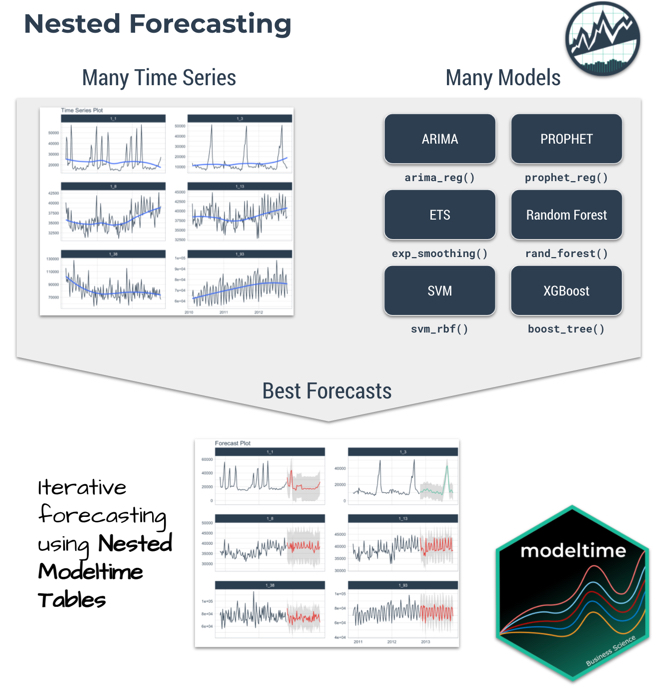
Iterative (Nested) Forecasting with Modeltime
We’ll show you how we can combine Modeltime “Nested Forecasting” and it’s Parallel Spark Backend to scale this computation with distributed parallel Spark execution.
Matt said “Nested”… What’s Nested?
A term that you’ll hear me use frequently is “nested”.
What I’m referring to is the “nested” data structure, which come from tidyr package that allows us to organize data frames as lists inside data frames. This is a powerful feature of the tidyverse that allows us for modeling at scale.
The book, “R for Data Science”, has a FULL Chapter on Many Models (and Nested Data). This is a great resource for those that want more info on Nested Data and Modeling (bookmark it ✅).
OK, let’s go!
System Requirements
This tutorial requires:
-
sparklyr, modeltime, and tidyverse: Make sure you have these R libraries installed (use install.packages(c("sparklyr", "modeltime", "tidyverse"), dependencies = TRUE)). If this is a fresh install, it may take a bit. Just be patient. ☕
-
Java: Spark installation depends on Java being installed. Download Java here.
-
Spark Installation: Can be accomplished via sparklyr::spark_install() provided the user has sparklyr and Java installed (see Steps 1 and 2).
Libraries
Load the following libraries.
library(sparklyr)
library(tidymodels)
library(modeltime)
library(tidyverse)
library(timetk)
Spark Connection
Next, we set up a Spark connection via sparklyr. For this tutorial, we use the “local” connection. But many users will use Databricks to scale the forecasting workload.
To run Spark locally:
sc <- spark_connect(master = "local")
If using Databricks, you can use:
sc <- spark_connect(method = "databricks")
Setup the Spark Backend
Next, we register the Spark Backend using parallel_start(sc, .method = "spark"). This is a helper to set up the registerDoSpark() foreach adaptor. In layman’s terms, this just means that we can now run parallel using Spark.
parallel_start(sc, .method = "spark")
Data Preparation (for Nested Forecasting)
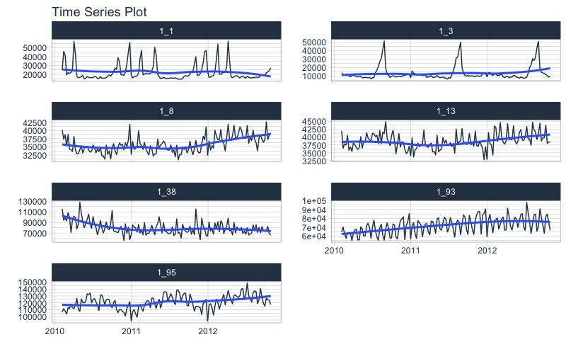
The dataset we’ll be forecasting is the walmart_sales_weekly, which we modify to just include 3 columns: “id”, “date”, “value”.
- The id feature is the grouping variable.
- The date feature contains timestamps.
- The value feature is the sales value for the Walmart store-department combination.
walmart_sales_weekly %>%
    select(id, Date, Weekly_Sales) %>%
    set_names(c("id", "date", "value")) %>%
    group_by(id) %>%
    plot_time_series(date, value, .facet_ncol = 2, .interactive = F)
We prepare as nested data using the Nested Forecasting preparation functions.
-
extend_timeseries(): This extends each one of our time series into the future by 52 timestamps (this is one year for our weekly data set).
-
nest_timeseries(): This converts our data to the nested data format indicating that our future data will be the last 52 timestamps (that we just extended).
-
split_nested_timeseries(): This adds indicies for the train / test splitting so we can develop accuracy metrics and determine which model to use for which time series.
nested_data_tbl <- walmart_sales_weekly %>%
    select(id, Date, Weekly_Sales) %>%
    set_names(c("id", "date", "value")) %>%
    extend_timeseries(
        .id_var        = id,
        .date_var      = date,
        .length_future = 52
    ) %>%
    nest_timeseries(
        .id_var        = id,
        .length_future = 52
    ) %>%

    split_nested_timeseries(
        .length_test = 52
    )

nested_data_tbl
## # A tibble: 7 × 4
##   id    .actual_data       .future_data      .splits
##   <fct> <list>             <list>            <list>
## 1 1_1   <tibble [143 × 2]> <tibble [52 × 2]> <split [91|52]>
## 2 1_3   <tibble [143 × 2]> <tibble [52 × 2]> <split [91|52]>
## 3 1_8   <tibble [143 × 2]> <tibble [52 × 2]> <split [91|52]>
## 4 1_13  <tibble [143 × 2]> <tibble [52 × 2]> <split [91|52]>
## 5 1_38  <tibble [143 × 2]> <tibble [52 × 2]> <split [91|52]>
## 6 1_93  <tibble [143 × 2]> <tibble [52 × 2]> <split [91|52]>
## 7 1_95  <tibble [143 × 2]> <tibble [52 × 2]> <split [91|52]>
Key Concept: Nested Data
You’ll notice our data frame (tibble) is only 7 rows and 4 columns. This is because we’ve nested our data.
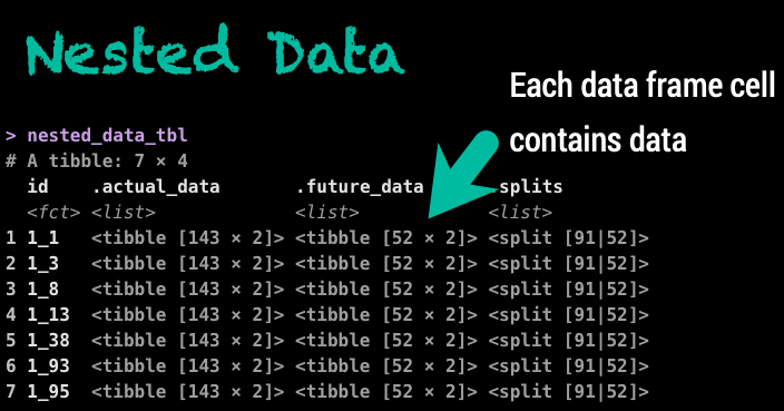
If you examine each of the rows, you’ll notice each row is an ID. And we have “tibbles” in each of the other columns.
That is nested data!
Modeling
We’ll create two unfitted models: XGBoost and Prophet. Then we’ll use modeltime_nested_fit() to iteratively fit the models to each of the time series using the Spark Backend.
Model 1: XGBoost
We create the XGBoost model on features derived from the date column. This gets a bit complicated because we are adding recipes to process the data. Basically, we are creating a bunch of features from the date column in each of the time series.
-
First, we use extract_nested_train_split(nested_data_tbl, 1) to extract the first time series, so we can begin to create a “recipe”
-
Once we develop a recipe, we add “steps” that build features. We start by creating timeseries signature features from the date column. Then we remove “date” and further process the signature features.
-
Then we create an XGBoost model by developing a tidymodels “workflow”. The workflow combines a model (boost_tree() in this case) with a recipe that we previously created.
-
The output is an unfitted workflow that will be applied to all 7 of our timeseries.
rec_xgb <- recipe(value ~ ., extract_nested_train_split(nested_data_tbl, 1)) %>%
    step_timeseries_signature(date) %>%
    step_rm(date) %>%
    step_zv(all_predictors()) %>%
    step_dummy(all_nominal_predictors(), one_hot = TRUE)

wflw_xgb <- workflow() %>%
    add_model(boost_tree("regression") %>% set_engine("xgboost")) %>%
    add_recipe(rec_xgb)

wflw_xgb
## ══ Workflow ════════════════════════════════════════════════════════════════════
## Preprocessor: Recipe
## Model: boost_tree()
##
## ── Preprocessor ────────────────────────────────────────────────────────────────
## 4 Recipe Steps
##
## • step_timeseries_signature()
## • step_rm()
## • step_zv()
## • step_dummy()
##
## ── Model ───────────────────────────────────────────────────────────────────────
## Boosted Tree Model Specification (regression)
##
## Computational engine: xgboost
Prophet
Next, we create a prophet workflow. The process is actually simpler than XGBoost because Prophet doesn’t require all of the preprocessing recipe steps that XGBoost does.
rec_prophet <- recipe(value ~ date, extract_nested_train_split(nested_data_tbl))

wflw_prophet <- workflow() %>%
    add_model(
        prophet_reg("regression", seasonality_yearly = TRUE) %>%
            set_engine("prophet")
    ) %>%
    add_recipe(rec_prophet)

wflw_prophet
## ══ Workflow ════════════════════════════════════════════════════════════════════
## Preprocessor: Recipe
## Model: prophet_reg()
##
## ── Preprocessor ────────────────────────────────────────────────────────────────
## 0 Recipe Steps
##
## ── Model ───────────────────────────────────────────────────────────────────────
## PROPHET Regression Model Specification (regression)
##
## Main Arguments:
##   seasonality_yearly = TRUE
##
## Computational engine: prophet
Nested Forecasting with Spark
Now, the beauty is that everything is set up for us to perform the nested forecasting with Spark. We simply use modeltime_nested_fit() and make sure it uses the Spark Backend by setting control_nested_fit(allow_par = TRUE).
Note that this will take about 20-seconds because we have a one-time cost to move data, libraries, and environment variables to the Spark clusters. But the good news is that when we scale up to 10,000+ time series, that the one-time cost is minimal compared to the speed up from distributed computation.
nested_modeltime_tbl <- nested_data_tbl %>%
    modeltime_nested_fit(
        wflw_xgb,
        wflw_prophet,

        control = control_nested_fit(allow_par = TRUE, verbose = TRUE)
    )
## Using existing parallel backend with 12 clusters (cores)...
##  Beginning Parallel Loop | 0.004 seconds
##  Finishing parallel backend. Clusters are remaining open. | 19.556 seconds
##  Close clusters by running: `parallel_stop()`.
##
## Finished in: 19.55732 secs.
The nested modeltime object has now fit the models using Spark. You’ll see a new column added to our nested data with the name “.modeltime_tables”. This contains 2 fitted models (one XGBoost and one Prophet) for each time series.
nested_modeltime_tbl
## # Nested Modeltime Table
##   # A tibble: 7 × 5
##   id    .actual_data       .future_data      .splits         .modeltime_tables
##   <fct> <list>             <list>            <list>          <list>
## 1 1_1   <tibble [143 × 2]> <tibble [52 × 2]> <split [91|52]> <mdl_time_tbl [2 ×…
## 2 1_3   <tibble [143 × 2]> <tibble [52 × 2]> <split [91|52]> <mdl_time_tbl [2 ×…
## 3 1_8   <tibble [143 × 2]> <tibble [52 × 2]> <split [91|52]> <mdl_time_tbl [2 ×…
## 4 1_13  <tibble [143 × 2]> <tibble [52 × 2]> <split [91|52]> <mdl_time_tbl [2 ×…
## 5 1_38  <tibble [143 × 2]> <tibble [52 × 2]> <split [91|52]> <mdl_time_tbl [2 ×…
## 6 1_93  <tibble [143 × 2]> <tibble [52 × 2]> <split [91|52]> <mdl_time_tbl [2 ×…
## 7 1_95  <tibble [143 × 2]> <tibble [52 × 2]> <split [91|52]> <mdl_time_tbl [2 ×…
Model Test Accuracy
We can observe the results. First, we can check the accuracy for each model.
nested_modeltime_tbl %>%
  extract_nested_test_accuracy() %>%
  table_modeltime_accuracy(.interactive = F)
| id |
.model_id |
.model_desc |
.type |
mae |
mape |
mase |
smape |
rmse |
rsq |
| 1_1 |
1 |
XGBOOST |
Test |
4552.91 |
18.14 |
0.90 |
17.04 |
7905.80 |
0.39 |
| 1_1 |
2 |
PROPHET |
Test |
4078.01 |
17.53 |
0.80 |
17.58 |
5984.31 |
0.65 |
| 1_3 |
1 |
XGBOOST |
Test |
1556.36 |
10.51 |
0.60 |
11.12 |
2361.35 |
0.94 |
| 1_3 |
2 |
PROPHET |
Test |
2126.56 |
13.15 |
0.83 |
13.91 |
3806.99 |
0.82 |
| 1_8 |
1 |
XGBOOST |
Test |
3573.49 |
9.31 |
1.52 |
9.87 |
4026.58 |
0.13 |
| 1_8 |
2 |
PROPHET |
Test |
3068.24 |
8.00 |
1.31 |
8.38 |
3639.60 |
0.00 |
| 1_13 |
1 |
XGBOOST |
Test |
2626.57 |
6.53 |
0.97 |
6.78 |
3079.24 |
0.43 |
| 1_13 |
2 |
PROPHET |
Test |
3367.92 |
8.26 |
1.24 |
8.73 |
4006.58 |
0.11 |
| 1_38 |
1 |
XGBOOST |
Test |
7865.35 |
9.62 |
0.67 |
10.14 |
10496.79 |
0.24 |
| 1_38 |
2 |
PROPHET |
Test |
16120.88 |
19.73 |
1.38 |
22.49 |
18856.72 |
0.05 |
| 1_93 |
1 |
XGBOOST |
Test |
6838.18 |
8.49 |
0.69 |
9.05 |
8860.59 |
0.48 |
| 1_93 |
2 |
PROPHET |
Test |
7304.08 |
10.00 |
0.74 |
9.57 |
9024.07 |
0.03 |
| 1_95 |
1 |
XGBOOST |
Test |
5678.51 |
4.59 |
0.68 |
4.72 |
7821.85 |
0.57 |
| 1_95 |
2 |
PROPHET |
Test |
5856.69 |
4.87 |
0.71 |
4.81 |
7540.48 |
0.49 |
Test Forecast
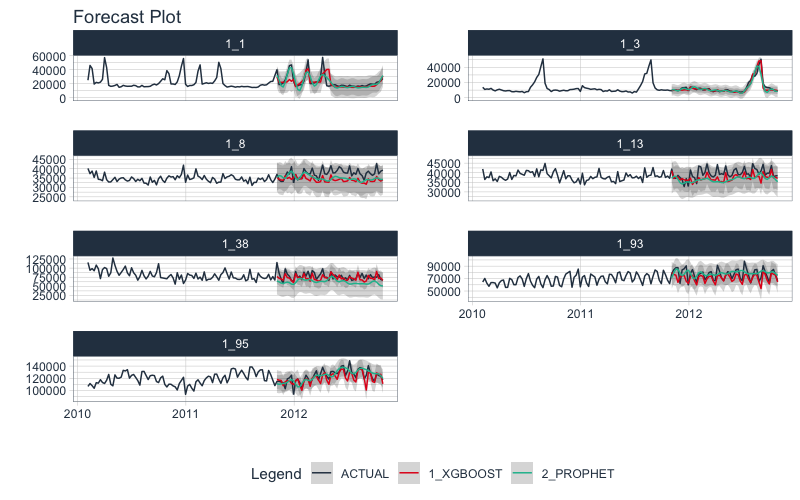
Next, we can examine the test forecast for each of the models.
-
We can use extract_nested_test_forecast() to extract the logged forecast and visualize how each did.
-
We group_by(id) then pipe (%>%) into plot_modeltime_forecast() to make the visualization (great for reports and shiny apps!)
nested_modeltime_tbl %>%
  extract_nested_test_forecast() %>%
  group_by(id) %>%
  plot_modeltime_forecast(.facet_ncol = 2, .interactive = F)
More we didn’t cover
There’s a lot more we didn’t cover. We actually didn’t:
- Select the best models for each of the 7 time series
- Improve performance with ensembles
- Forecast the future
I’ll cover these and much more in the Free Live Training on Forecasting with Spark.
Make sure to sign up and you’ll get 3 immediately actionable tips and a full code tutorial that goes well beyond this introduction.
Plus you’ll get exclusive offers on our courses and get to ask me (Matt, the creator of Modeltime) questions!
Close Clusters and Shutdown Spark
We can close the Spark adapter and shut down the Spark session when we are finished.
# Unregisters the Spark Backend
parallel_stop()

# Disconnects Spark
spark_disconnect_all()
## [1] 1
Summary
We’ve now successfully completed an Forecast with Spark. You may find this challenging, especially if you are not familiar with the Modeltime Workflow, terminology, or tidymodeling in R. If this is the case, we have a solution. Take our high-performance forecasting course.
Become the forecasting expert for your organization
High-Performance Time Series Course
Time Series is Changing
Time series is changing. Businesses now need 10,000+ time series forecasts every day. This is what I call a High-Performance Time Series Forecasting System (HPTSF) - Accurate, Robust, and Scalable Forecasting.
High-Performance Forecasting Systems will save companies by improving accuracy and scalability. Imagine what will happen to your career if you can provide your organization a “High-Performance Time Series Forecasting System” (HPTSF System).
I teach how to build a HPTFS System in my High-Performance Time Series Forecasting Course. You will learn:
- Time Series Machine Learning (cutting-edge) with
Modeltime - 30+ Models (Prophet, ARIMA, XGBoost, Random Forest, & many more)
- Deep Learning with
GluonTS (Competition Winners)
- Time Series Preprocessing, Noise Reduction, & Anomaly Detection
- Feature engineering using lagged variables & external regressors
- Hyperparameter Tuning
- Time series cross-validation
- Ensembling Multiple Machine Learning & Univariate Modeling Techniques (Competition Winner)
- Scalable Forecasting - Forecast 1000+ time series in parallel
- and more.
Become the Time Series Expert for your organization.
Take the High-Performance Time Series Forecasting Course