How to Set Up TensorFlow 2 in R in 5 Minutes (BONUS Image Recognition Tutorial)
Written by Matt Dancho

The 2 most popular data science languages - Python and R - are often pitted as rivals. This couldn’t be further from the truth. Data scientists that learn to use the strengths of both languages are valuable because they have NO LIMITS.
- Machine Learning and Deep Learning: They can switch to Python to leverage
scikit learn and tensorflow.
- Data Wrangling, Visualization, Apps & Reporting: They can quickly change to R to use
tidyverse, shiny and rmarkdown.
The bottom line is that knowing both R and Python makes you SUPER PRODUCTIVE.
Article Updates:
Have 5 minutes?
Then let’s set up TensorFlow 2 for Deep Learning
TensorFlow in R!
We’re going to go through the essential setup tips of the PRO’s - those that use Python from R via reticulate.
Here’s the BONUS Image Reconition Tutorial. You’ll classify Fashion Images.
TensorFlow Ankle Boot Classification - Tutorial to Test if TF is Working
Using TensorFlow & R
How do you use them together in Business Projects?
Setting up TensorFlow in R is an insane productivity booster. You can leverage the best of Python + R. But you still need to learn how to use Python and R together for real business projects. And, it’s impossible to teach you all the in’s and out’s in 1 short article. But, I have great news!
I just launched a NEW 5-PART PYTHON + R LEARNING LAB SERIES (Register Here) that will show you how to use Python and R together on Real Business Projects:
- Lab 33: Human Resources Employee Segmentation
- Lab 34: Advanced Customer Segmentation and Market Basket Analysis
- Lab 35: TensorFlow for Finance
- Lab 36: TensorFlow for Energy Demand Forecasting
- Lab 37: Social Media Text Analytics!
And it’s FREE to attend live.
Register here to attend Python + R Learning Labs live for free. I’ll notify you in advance of the accelerated 1-hour courses that you can attend via webinar.
Installing TensorFlow in R
This process should take under 5-minutes. First we have some requirments to get TensorFlow 2 installed.
TensorFlow 2.0.0 Requirements
These may (will) change in the future, but currently the requirements are:
- Python 3.5-3.7
- Windows 7 or Later
- MacOS 10.12.6 or Later
- Ubunto 16.04 or Later
If you’ve followed the Scikit Learn in R tutorial, we used Python 3.8 (latest stable version). We can’t use Python 3.8 for TensorFlow, so we need to create a new environment. We’ll use Python 3.6 in this tutorial.
Conda Requirements
If you don’t have Conda installed, please install here: Anaconda Installation.
Installing TensorFlow in R with reticulate
Do this in R. Install and load tidyverse, reticulate, and tensorflow.
# R
library(tidyverse)
library(reticulate)
library(tensorflow)
Next, run install_tensorflow() in your R environment. This will take about 3-5 minutes to install TensorFlow in a new Conda Environment named “py3.6”.
# R
install_tensorflow(
    method               = "conda",
    version              = "default", # Installs TF 2.0.0 (as of May 15, 2020)
    envname              = "py3.6",
    conda_python_version = "3.6",
    extra_packages       = c("matplotlib", "numpy", "pandas", "scikit-learn")
)
Side note: You can actually specify which TensorFlow version to install with the version arg. This can be helpful to switch from the CPU vesion to GPU version (greater power, greater responsibility) or to access older versions of TF.
We can check to see that py3.6 conda environment has been created.
# R
conda_list()
##        name                                             python
## 1 anaconda3            /Users/mdancho/opt/anaconda3/bin/python
## 2     py3.6 /Users/mdancho/opt/anaconda3/envs/py3.6/bin/python
## 3     py3.7 /Users/mdancho/opt/anaconda3/envs/py3.7/bin/python
## 4     py3.8 /Users/mdancho/opt/anaconda3/envs/py3.8/bin/python
Next, we tell reticulate to use the py3.6 conda environment.
# R
use_condaenv("py3.6", required = TRUE)
Congrats on the Installation is now complete! - Now Let’s Use TensorFlow to classify images.
Image Recognition Analysis
To Verify TensorFlow is Working
Let’s run through a short image recognition tutorial. This tutorial comes from Google’s Basic classification: Classify images of clothing
Step 1 - Make a Python Code Chunk
Use Pro-Tip #1 Below to make a “Python Code Chunk”.
Python Code Chunk
Step 2 - Import Libraries
Import the libraries needed:
- Deep Learning:
tensorflow and keras
- Math:
numpy
- Visualization:
matplotlib
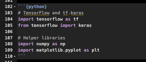
# Python

# TensorFlow and tf.keras
import tensorflow as tf
from tensorflow import keras

# Helper libraries
import numpy as np
import matplotlib.pyplot as plt
Check the version of tensorflow to make sure we’re using 2.0.0+.
# Python
print(tf.__version__)
## 2.0.0
Step 3 - Load the Fashion Images
Load the fashion_mnist dataset from keras.
# Python
fashion_mnist = keras.datasets.fashion_mnist

(train_images, train_labels), (test_images, test_labels) = fashion_mnist.load_data()
We have 60,000 training images that have been labeled.
# Python
train_images.shape
## (60000, 28, 28)
We can check the unique labels to see what classifications the images belong to. Note that these are numeric values ranging from 0 to 9.
# Python
np.unique(train_labels)
## array([0, 1, 2, 3, 4, 5, 6, 7, 8, 9], dtype=uint8)
The corresponding labels are:
# Python
class_names = ['T-shirt/top', 'Trouser', 'Pullover', 'Dress', 'Coat',
               'Sandal', 'Shirt', 'Sneaker', 'Bag', 'Ankle boot']
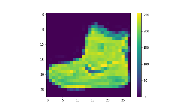
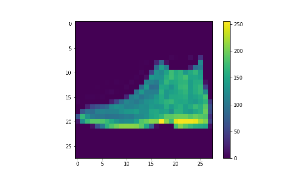
We can see what the first image looks like using matplotlib.
# Python
plt.figure()
plt.imshow(train_images[0])
plt.colorbar()
plt.grid(False)
plt.show()
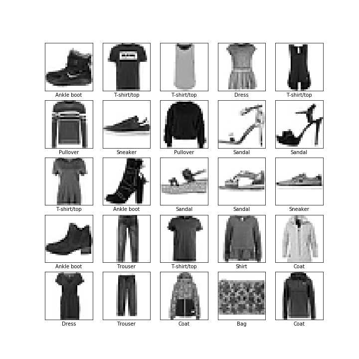
And we can also check out the first 25 images.
# Python
plt.figure(figsize=(10,10))
for i in range(25):
    plt.subplot(5,5,i+1)
    plt.xticks([])
    plt.yticks([])
    plt.grid(False)
    plt.imshow(train_images[i], cmap=plt.cm.binary)
    plt.xlabel(class_names[train_labels[i]])
plt.show()
Step 4 - Modeling with Keras
Make a keras model using the Sequential() with 3 steps: Flatten, Dense, and Dense.
# Python
model = keras.Sequential([
    keras.layers.Flatten(input_shape=(28, 28)),
    keras.layers.Dense(128, activation='relu'),
    keras.layers.Dense(10)
])
Next, compile the model with the “adam” optimizer.
# Python
model.compile(
    optimizer = 'adam',
    loss      = tf.keras.losses.SparseCategoricalCrossentropy(from_logits=True),
    metrics   = ['accuracy']
)
Inspect the model summary.
# Python
model.summary()
## Model: "sequential"
## _________________________________________________________________
## Layer (type)                 Output Shape              Param #
## =================================================================
## flatten (Flatten)            (None, 784)               0
## _________________________________________________________________
## dense (Dense)                (None, 128)               100480
## _________________________________________________________________
## dense_1 (Dense)              (None, 10)                1290
## =================================================================
## Total params: 101,770
## Trainable params: 101,770
## Non-trainable params: 0
## _________________________________________________________________
Step 5 - Fit the Keras Model
CRITICAL STEP - Fit the model. Make sure this step works!</p>
# Python
model.fit(train_images, train_labels, epochs=10, verbose=1)
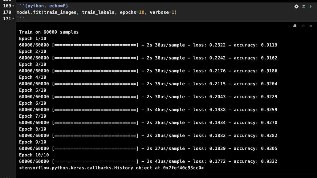
TensorFlow Model Training
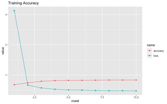
Step 6 - Training History
# Python
history = model.history.history
history
## {'loss': [3.1226694132328032, 0.6653605920394262, 0.5747007430752118, 0.5286751741568247, 0.508751327864329, 0.5023731174985567, 0.48900006746848423, 0.4814090680360794, 0.4810072046995163, 0.47561218699614205], 'accuracy': [0.68145, 0.74085, 0.79331666, 0.8143, 0.8228833, 0.8244333, 0.8283167, 0.83428335, 0.8348, 0.83521664]}
I’ll plot this using R. Note - This is an R Code Chunk (not a Python Code Chunk).
# R Code Chunk (not Python)
py$history %>%
    as_tibble() %>%
    unnest(loss, accuracy) %>%
    rowid_to_column() %>%
    pivot_longer(-rowid) %>%
    ggplot(aes(rowid, value, color = name)) +
    geom_line() +
    geom_point() +
    labs(title = "Training Accuracy")
Step 7 - Test Accuracy
Evaluate accuracy on the out-of-sample images.
# Python
test_loss, test_acc = model.evaluate(test_images,  test_labels, verbose=2)
## 10000/1 - 0s - loss: 0.4470 - accuracy: 0.8098
Step 8 - Make Predictions
The model produces linear outputs cakked “logits”. The softmax layer to converts the logits to probabilities.
# Python
probability_model = tf.keras.Sequential([model, tf.keras.layers.Softmax()])
We can then classify all of the test images (held out)
# Python
predictions = probability_model.predict(test_images)
We can make a prediction for the first image.
# Python
predictions[0]
## array([7.7921860e-21, 3.3554016e-13, 0.0000000e+00, 1.8183892e-15,
##        0.0000000e+00, 4.0730215e-03, 8.1443369e-20, 4.2793788e-03,
##        2.6940727e-18, 9.9164760e-01], dtype=float32)
Use np.argmax() to determine which index has the highest probability.
# Python
np.argmax(predictions[0])
## 9
The index value can be retrieved with np.max().
# Python
np.max(predictions[0])
## 0.9916476
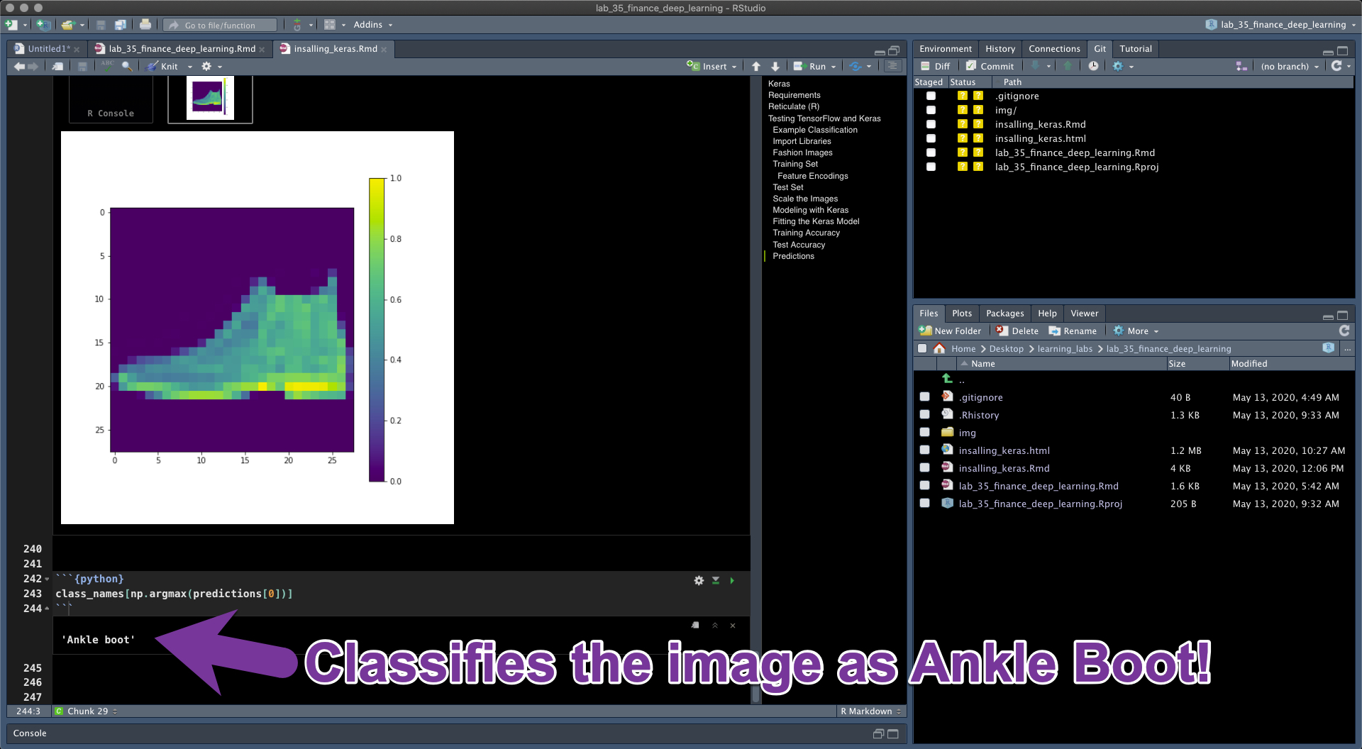
Get the class name.
# Python
class_names[np.argmax(predictions[0])]
## 'Ankle boot'
And visualize the image.
# Python
plt.figure()
plt.imshow(test_images[0])
plt.colorbar()
## <matplotlib.colorbar.Colorbar object at 0x7fee14906240>
# Python
plt.grid(False)
plt.show()
Nice work - If you made it through this tutorial unscathed, then you are doing well! And your ready for the TensorFlow Learning Labs.
Pro Tips (Python in R)
Now that you have python running in R, use these pro-tips to make your experience way more enjoyable.
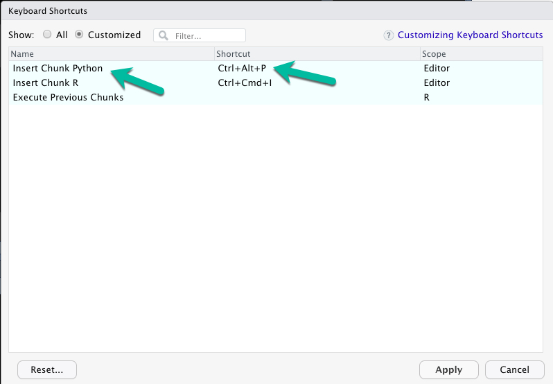
Pro-Tip #1 - Python Chunk Keyboard Shortcut
I can’t stress this one enough - Set up a Keyboard shortcut for Python Code Chunks. This is a massive productivity booster for Rmarkdown documents.
- My preference:
Ctrl + Alt + P
When you hit Ctrl + Alt + P, a {python} code chunk will appear in your R Markdown document.
Pro-Tip #2 - Use Python Interactively
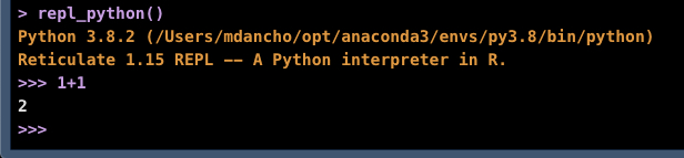
For debugging Python Code Chunks in R Markdown, it can help to use the repl_python() to convert your Console to a Python Code Console. To do so:
- In R Console, you can run python interactively using
repl_python(). You will see >>> indicating you are in Python Mode.
- Make sure the correct Python / Conda Environment is selected.
- To escape Python in the console, just hit
escape.
Pro-Tip #3 - My Top 4 Conda Terminal Commands
At some point you will need to create, modify, add more packages to your Conda Environment(s). Here are 4 useful commands:
- Run
conda env list to list the available conda environments
- Run
conda activate <env_name> to activate a conda environment
- Run
conda update --all to update all python packages in a conda environment.
- Run
conda install <package_name> to install a new package
Use Python inside Shiny Apps
Up until now we haven’t talked about Shiny - the web application framework that is used to take your python and R machine learning models into Production.

Business Science Application Library
A Meta-Application that houses Shiny Apps
R Shiny needs to be in your toolbox if you want to productionize Data Science. You simply cannot put machine learning applications into production with other “BI” Tools like Tableau, PowerBI, and QlikView.
CRITICAL POINT: You can USE SHINY to productionize Scikit Learn and TensorFlow models.
If you need to learn R Shiny as fast as possible, I have the perfect program for you. It will accelerate your career. The 4-Course R-Track Bundle through Business Science.
Have questions on using Python + R?
Make a comment in the chat below. 👇
And, if you plan on using Python + R at work, it’s a no-brainer - attend my Learning Labs (they are FREE to attend live).