Introducing Iterative (Nested) Forecasting with Modeltime
Written by Matt Dancho
Iteratively forecast with tidyverse nested modeling
Why is nested forecasting important? For starters, the ability to iteratively forecast time series with many models that are trained on many individual groups has been a huge request from students in our Time Series Course.
Two methods exist for forecasting many time series that get results:
-
Global Modeling: Best for scalability using a Global Models and Panel Data structure. See Forecasting with Global Models.
-
Iterative Forecasting: Best for accuracy using a Nested Data Structure. Takes longer than global model (more resources due to for-loop iteration), but can yield great results. (Discussed Here)
We’ve incorporated a new approach called “Nested Forecasting” to help perform Iterative Forecasting inside of a tidyverse nested data structure. You’ll scalably create 7 prophet and 7 xgboost models.
If you like what you see, I have an Advanced Time Series Course where you will learn the foundations of the growing Modeltime Ecosystem.
Before we get started, install modeltime
The new nested forecasting is only available in the development version of modeltime. We will be releasing to CRAN soon.
For now, you can install with:
remotes::install_github("business-science/modeltime", dependencies = TRUE)
What is Modeltime?
A growing ecosystem for tidymodels forecasting
Modeltime is part of a growing ecosystem of forecasting packages. Modeltime integrates tidymodels for forecasting at scale. The ecosystem contains:
And several new community-contributed modeltime extension packages have emerged including: boostime, bayesmodels, garchmodels, and sknifedatar
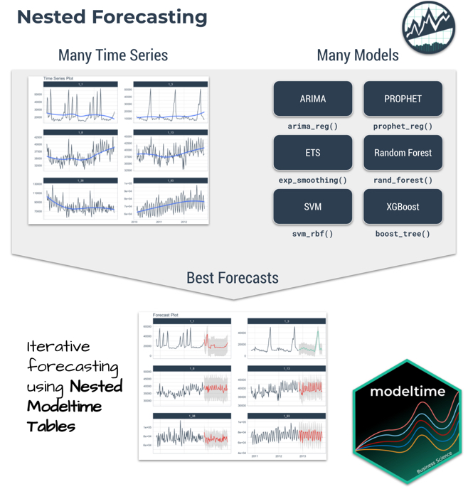
What is Nested Forecasting?
Nested forecasting is a new feature in modeltime. The core idea of nested forecasting is to convert a dataset containing many time series groups into a nested data set, then fit many models to each of the nested data sets. The result is an iterative forecasting process that generates Nested Modeltime Tables with all of the forecast attributes needed to make decisions.
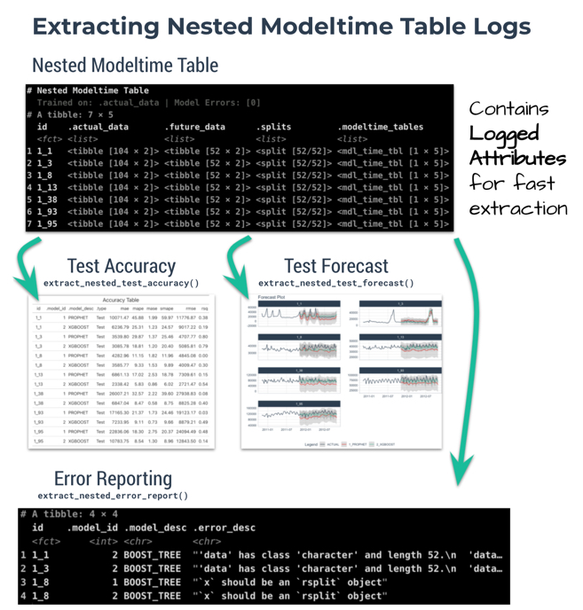
Important Concepts: Logging & Attributes
A new feature to nested forecasting workflow is logged attributes, which is very useful in complex workflows where loops (iteration) is performed. In a Nested Modeltime Table, we push as many operations as possible into the fitting and refitting stages, logging important aspects including:
- Test Accuracy:
extract_nested_test_accuracy()
- Test Forecast:
extract_nested_test_forecast()
- Error Reports:
extract_nested_error_report()
- Best Models:
extract_nested_best_model_report()
- Future Forecasts:
extract_nested_future_forecast()
While this deviates from the traditional Modeltime Workflow, we find that logging vastly speeds up experimentation and information retrieval especially when the number of time series increases.
Getting Started
We’ll go through a short tutorial on Nested Forecasting. The first thing to do is to load the following libraries:
library(tidymodels)
library(modeltime)
library(tidyverse)
library(timetk)
Dataset
Next, let’s use the walmart_sales_weekly dataset that comes with timetk.
data_tbl <- walmart_sales_weekly %>%
    select(id, Date, Weekly_Sales) %>%
    set_names(c("id", "date", "value"))

data_tbl
## # A tibble: 1,001 × 3
##    id    date        value
##    <fct> <date>      <dbl>
##  1 1_1   2010-02-05 24924.
##  2 1_1   2010-02-12 46039.
##  3 1_1   2010-02-19 41596.
##  4 1_1   2010-02-26 19404.
##  5 1_1   2010-03-05 21828.
##  6 1_1   2010-03-12 21043.
##  7 1_1   2010-03-19 22137.
##  8 1_1   2010-03-26 26229.
##  9 1_1   2010-04-02 57258.
## 10 1_1   2010-04-09 42961.
## # … with 991 more rows
The problem with this dataset is that it’s set up for panel data modeling.
The important columns are:
-
“id”: This separates the time series groups (in this case these represent sales from departments in a walmart store)
-
“date”: This is the weekly sales period
-
“value”: This is the value for sales during the week and store/department
We can visualize the sales data by time series group (department ID) to expose the differences in sales by department.
data_tbl %>%
  group_by(id) %>%
  plot_time_series(
    date, value, .interactive = F, .facet_ncol = 2
  )
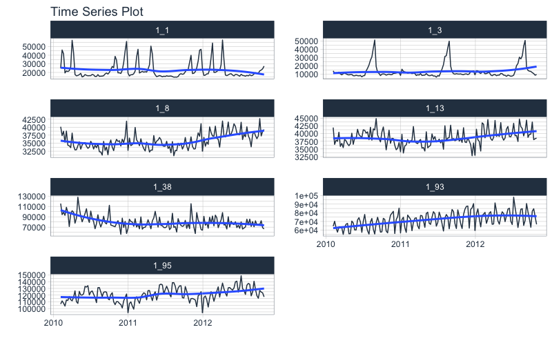
We can clearly see that there are 7 time series groups (store departments) with different weekly sales patterns.
Nested Forecasting Preparation
There are two key components that we need to prepare for:
-
Nested Data Structure: Most critical to ensure your data is prepared (covered next)
-
Nested Modeltime Workflow: This stage is where we create many models, fit the models to the data, and generate forecasts at scale
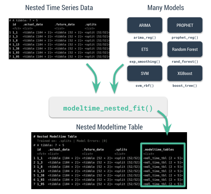
Conceptually, the workflow looks like this where we combine nested data and tidymodels workflows using an upcoming function, modeltime_nested_fit().
Data Preparation (Nesting)
The most critical stage in “Nested Forecasting” is data preparation, making sure that the input to the nested forecasting workflow is in the appropriate structure. We’ve included several functions to help that involve a bit of forethought that can be broken into 3 steps:
-
Extending each of the times series: How far into the future do you need to predict for each time series? See extend_timeseries().
-
Nesting by the grouping variable: This is where you create the nested structure. You’ll identify the ID column that separates each time series, and the number of timestamps to include in the “.future_data” and optionally “.actual_data”. Typically, you’ll select the same .length_future as your extension from the previous step. See nest_timeseries().
-
Train/Test Set Splitting: Finally, you’ll take your .actual_data and convert into train/test splits that can be used for accuracy and confidence interval estimation. See split_nested_timeseries().
Here are the 3-steps in action:
nested_data_tbl <- data_tbl %>%

    # 1. Extending: We'll predict 52 weeks into the future.
    extend_timeseries(
        .id_var        = id,
        .date_var      = date,
        .length_future = 52
    ) %>%

    # 2. Nesting: We'll group by id, and create a future dataset
    #    that forecasts 52 weeks of extended data and
    #    an actual dataset that contains 104 weeks (2-years of data)
    nest_timeseries(
        .id_var        = id,
        .length_future = 52,
        .length_actual = 52*2
    ) %>%

   # 3. Splitting: We'll take the actual data and create splits
   #    for accuracy and confidence interval estimation of 52 weeks (test)
   #    and the rest is training data
    split_nested_timeseries(
        .length_test = 52
    )

nested_data_tbl
## # A tibble: 7 × 4
##   id    .actual_data       .future_data      .splits
##   <fct> <list>             <list>            <list>
## 1 1_1   <tibble [104 × 2]> <tibble [52 × 2]> <split [52/52]>
## 2 1_3   <tibble [104 × 2]> <tibble [52 × 2]> <split [52/52]>
## 3 1_8   <tibble [104 × 2]> <tibble [52 × 2]> <split [52/52]>
## 4 1_13  <tibble [104 × 2]> <tibble [52 × 2]> <split [52/52]>
## 5 1_38  <tibble [104 × 2]> <tibble [52 × 2]> <split [52/52]>
## 6 1_93  <tibble [104 × 2]> <tibble [52 × 2]> <split [52/52]>
## 7 1_95  <tibble [104 × 2]> <tibble [52 × 2]> <split [52/52]>
This creates a nested tibble with “.actual_data”, “.future_data”, and “.splits”. Each column will help in the nested modeltime workflow.
Nested Modeltime Workflow
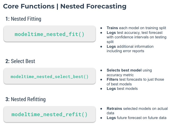
Next, we move into the Nested Modeltime Workflow now that nested data has been created. The Nested Modeltime Workflow includes 3 core functions:
-
Modeling Fitting: This is the training stage where we fit to training data. The test forecast is generated from this step. See modeltime_nested_fit().
-
Model Evaluation and Selection: This is where we review model performance and select the best model by minimizing or maximizing an error metric. See modeltime_nested_select_best().
-
Model Refitting: This is the final fitting stage where we fit to actual data. The future forecast is generated from this step. See modeltime_nested_refit().
Step 1: Create Tidymodels Workflows
First, we create tidymodels workflows for the various models that you intend to create.
Prophet
A common modeling method is prophet, that can be created using prophet_reg(). We’ll create a workflow. Note that we use the extract_nested_train_split(nested_data_tbl) to help us build preprocessing features.
rec_prophet <- recipe(value ~ date,  extract_nested_train_split(nested_data_tbl))

wflw_prophet <- workflow() %>%
    add_model(
      prophet_reg("regression", seasonality_yearly = TRUE) %>%
        set_engine("prophet")
    ) %>%
    add_recipe(rec_prophet)
XGBoost
Next, we can use a machine learning method that can get good results: XGBoost. We will add a few extra features in the recipe feature engineering step to generate features that tend to get better modeling results. Note that we use the extract_nested_train_split(nested_data_tbl) to help us build preprocessing features.
rec_xgb <- recipe(value ~ .,  extract_nested_train_split(nested_data_tbl)) %>%
    step_timeseries_signature(date) %>%
    step_rm(date) %>%
    step_zv(all_predictors()) %>%
    step_dummy(all_nominal_predictors(), one_hot = TRUE)

wflw_xgb <- workflow() %>%
    add_model(boost_tree("regression") %>% set_engine("xgboost")) %>%
    add_recipe(rec_xgb)
Step 2: Nested Modeltime Tables
With a couple of modeling workflows in hand, we are now ready to test them on each of the time series. We start by using the modeltime_nested_fit() function, which iteratively fits each model to each of the nested time series train/test “.splits” column.
nested_modeltime_tbl <- modeltime_nested_fit(
  # Nested data
  nested_data = nested_data_tbl,

  # Add workflows
  wflw_prophet,
  wflw_xgb
)

nested_modeltime_tbl
## # Nested Modeltime Table
## # Trained on: .splits | Model Errors: [0]
## # A tibble: 7 × 5
##   id    .actual_data       .future_data     .splits        .modeltime_tables
##   <fct> <list>             <list>           <list>         <list>
## 1 1_1   <tibble [104 × 2]> <tibble [52 × 2… <split [52/52… <mdl_time_tbl [2 × 5…
## 2 1_3   <tibble [104 × 2]> <tibble [52 × 2… <split [52/52… <mdl_time_tbl [2 × 5…
## 3 1_8   <tibble [104 × 2]> <tibble [52 × 2… <split [52/52… <mdl_time_tbl [2 × 5…
## 4 1_13  <tibble [104 × 2]> <tibble [52 × 2… <split [52/52… <mdl_time_tbl [2 × 5…
## 5 1_38  <tibble [104 × 2]> <tibble [52 × 2… <split [52/52… <mdl_time_tbl [2 × 5…
## 6 1_93  <tibble [104 × 2]> <tibble [52 × 2… <split [52/52… <mdl_time_tbl [2 × 5…
## 7 1_95  <tibble [104 × 2]> <tibble [52 × 2… <split [52/52… <mdl_time_tbl [2 × 5…
This adds a new column with .modeltime_tables for each of the data sets and has created several logged attributes that are part of the “Nested Modeltime Table”. We also can see that the models were trained on “.splits” and none of the models had any errors.
Step 3: Logged Attributes
During the forecasting, the iterative modeltime fitting process logs important information that enable us to evaluate the models. These logged attributes are accessable with “extract” functions.
Using the extract_nested_test_accuracy(), we can get the accuracy measures by time series and model. This allows us to see which model performs best on which time series.
nested_modeltime_tbl %>%
  extract_nested_test_accuracy() %>%
  table_modeltime_accuracy(.interactive = F)
| id |
.model_id |
.model_desc |
.type |
mae |
mape |
mase |
smape |
rmse |
rsq |
| 1_1 |
1 |
PROPHET |
Test |
10071.47 |
45.88 |
1.99 |
59.97 |
11776.87 |
0.38 |
| 1_1 |
2 |
XGBOOST |
Test |
6236.79 |
25.31 |
1.23 |
24.57 |
9017.22 |
0.19 |
| 1_3 |
1 |
PROPHET |
Test |
3539.80 |
29.87 |
1.37 |
25.46 |
4707.77 |
0.80 |
| 1_3 |
2 |
XGBOOST |
Test |
3085.78 |
18.81 |
1.20 |
20.40 |
5085.81 |
0.79 |
| 1_8 |
1 |
PROPHET |
Test |
4282.96 |
11.15 |
1.82 |
11.96 |
4845.08 |
0.00 |
| 1_8 |
2 |
XGBOOST |
Test |
3585.77 |
9.33 |
1.53 |
9.89 |
4009.47 |
0.30 |
| 1_13 |
1 |
PROPHET |
Test |
6861.13 |
17.02 |
2.53 |
18.78 |
7309.61 |
0.15 |
| 1_13 |
2 |
XGBOOST |
Test |
2338.42 |
5.83 |
0.86 |
6.02 |
2721.47 |
0.54 |
| 1_38 |
1 |
PROPHET |
Test |
26007.21 |
32.57 |
2.22 |
39.60 |
27938.83 |
0.08 |
| 1_38 |
2 |
XGBOOST |
Test |
6847.04 |
8.47 |
0.58 |
8.75 |
8825.28 |
0.40 |
| 1_93 |
1 |
PROPHET |
Test |
17165.30 |
21.37 |
1.73 |
24.46 |
19123.17 |
0.03 |
| 1_93 |
2 |
XGBOOST |
Test |
7233.95 |
9.11 |
0.73 |
9.66 |
8879.21 |
0.49 |
| 1_95 |
1 |
PROPHET |
Test |
22836.06 |
18.30 |
2.75 |
20.37 |
24094.49 |
0.48 |
| 1_95 |
2 |
XGBOOST |
Test |
10783.75 |
8.54 |
1.30 |
8.96 |
12843.50 |
0.14 |
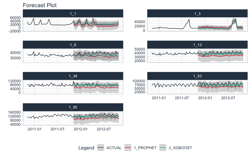
Next, we can visualize the test forecast with extract_nested_test_forecast().
nested_modeltime_tbl %>%
  extract_nested_test_forecast() %>%
  group_by(id) %>%
  plot_modeltime_forecast(
    .facet_ncol  = 2,
    .interactive = FALSE
  )
If any of the models have errors, then we can investigate the error logs with extract_nested_error_report(). Fortunately, we don’t have any errors, but if we did we could investigate further.
nested_modeltime_tbl %>%
  extract_nested_error_report()
## # A tibble: 0 × 4
## # … with 4 variables: id <fct>, .model_id <int>, .model_desc <chr>,
## #   .error_desc <chr>
Step 4: Select the Best
Using the accuracy data, we can pick a metric and select the best model based on that metric. The available metrics are in the default_forecast_accuracy_metric_set(). Make sure to select minimize based on the metric. The filter_test_forecasts parameter tells the function to filter the logged test forecasts to just the best.
best_nested_modeltime_tbl <- nested_modeltime_tbl %>%
            modeltime_nested_select_best(
              metric                = "rmse",
              minimize              = TRUE,
              filter_test_forecasts = TRUE
            )
This identifies which models should be used for the final forecast. With the models selected, we can make the future forecast.
The best model selections can be accessed with extract_nested_best_model_report().
best_nested_modeltime_tbl %>%
  extract_nested_best_model_report()
## # Nested Modeltime Table
##   # A tibble: 7 × 10
##   id    .model_id .model_desc .type    mae  mape  mase smape   rmse   rsq
##   <fct>     <int> <chr>       <chr>  <dbl> <dbl> <dbl> <dbl>  <dbl> <dbl>
## 1 1_1           2 XGBOOST     Test   6237. 25.3  1.23  24.6   9017. 0.191
## 2 1_3           1 PROPHET     Test   3540. 29.9  1.37  25.5   4708. 0.796
## 3 1_8           2 XGBOOST     Test   3586.  9.33 1.53   9.89  4009. 0.297
## 4 1_13          2 XGBOOST     Test   2338.  5.83 0.861  6.02  2721. 0.536
## 5 1_38          2 XGBOOST     Test   6847.  8.47 0.585  8.75  8825. 0.402
## 6 1_93          2 XGBOOST     Test   7234.  9.11 0.728  9.66  8879. 0.488
## 7 1_95          2 XGBOOST     Test  10784.  8.54 1.30   8.96 12843. 0.139
Once we’ve selected the best models, we can easily visualize the best forecasts by time series. Note that the nested test forecast logs have been modified to isolate the best models.
best_nested_modeltime_tbl %>%
  extract_nested_test_forecast() %>%
  group_by(id) %>%
  plot_modeltime_forecast(
    .facet_ncol  = 2,
    .interactive = FALSE
  )

Step 5: Refitting and Future Forecast
With the best models in hand, we can make our future forecasts by refitting the models to the full dataset.
-
If the best models have been selected, the only the best models will be refit.
-
If best models have not been selected, then all models will be refit.
We’ve selected our best models, and will move forward with refitting and future forecast logging using the modeltime_nested_refit() function.
nested_modeltime_refit_tbl <- best_nested_modeltime_tbl %>%
    modeltime_nested_refit(
        control = control_nested_refit(verbose = TRUE)
    )

## ℹ [1/7] Starting Modeltime Table: ID 1_1...
## ✓ Model 2 Passed XGBOOST.
## ✓ [1/7] Finished Modeltime Table: ID 1_1

## ℹ [2/7] Starting Modeltime Table: ID 1_3...
## ✓ Model 1 Passed PROPHET.
## ✓ [2/7] Finished Modeltime Table: ID 1_3

## ℹ [3/7] Starting Modeltime Table: ID 1_8...
## ✓ Model 2 Passed XGBOOST.
## ✓ [3/7] Finished Modeltime Table: ID 1_8

## ℹ [4/7] Starting Modeltime Table: ID 1_13...
## ✓ Model 2 Passed XGBOOST.
## ✓ [4/7] Finished Modeltime Table: ID 1_13

## ℹ [5/7] Starting Modeltime Table: ID 1_38...
## ✓ Model 2 Passed XGBOOST.
## ✓ [5/7] Finished Modeltime Table: ID 1_38

## ℹ [6/7] Starting Modeltime Table: ID 1_93...
## ✓ Model 2 Passed XGBOOST.
## ✓ [6/7] Finished Modeltime Table: ID 1_93

## ℹ [7/7] Starting Modeltime Table: ID 1_95...
## ✓ Model 2 Passed XGBOOST.
## ✓ [7/7] Finished Modeltime Table: ID 1_95

## Finished in: 3.52616 secs.
Note that we used control_nested_refit(verbose = TRUE) to display the modeling results as each model is refit. This is not necessary, but can be useful to follow the nested model fitting process.
We can see that the nested modeltime table appears the same, but has now been trained on .actual_data.
nested_modeltime_refit_tbl

## # Nested Modeltime Table
## # Trained on: .actual_data | Model Errors: [0]
## # A tibble: 7 × 5
##   id    .actual_data       .future_data     .splits        .modeltime_tables
##   <fct> <list>             <list>           <list>         <list>
## 1 1_1   <tibble [104 × 2]> <tibble [52 × 2… <split [52/52… <mdl_time_tbl [1 × 5…
## 2 1_3   <tibble [104 × 2]> <tibble [52 × 2… <split [52/52… <mdl_time_tbl [1 × 5…
## 3 1_8   <tibble [104 × 2]> <tibble [52 × 2… <split [52/52… <mdl_time_tbl [1 × 5…
## 4 1_13  <tibble [104 × 2]> <tibble [52 × 2… <split [52/52… <mdl_time_tbl [1 × 5…
## 5 1_38  <tibble [104 × 2]> <tibble [52 × 2… <split [52/52… <mdl_time_tbl [1 × 5…
## 6 1_93  <tibble [104 × 2]> <tibble [52 × 2… <split [52/52… <mdl_time_tbl [1 × 5…
## 7 1_95  <tibble [104 × 2]> <tibble [52 × 2… <split [52/52… <mdl_time_tbl [1 × 5…
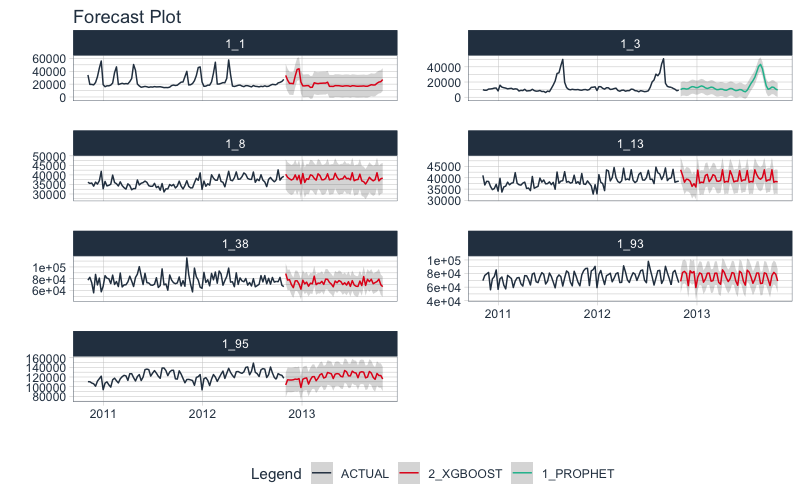
After the refitting process completes, we can now access the future forecast, which is logged.
nested_modeltime_refit_tbl %>%
  extract_nested_future_forecast() %>%
  group_by(id) %>%
  plot_modeltime_forecast(
    .interactive = FALSE,
    .facet_ncol  = 2
  )
Summary
We’ve now successfully completed a Nested Forecast. You may find this challenging, especially if you are not familiar with the Modeltime Workflow, terminology, or tidymodeling in R. If this is the case, we have a solution. Take our high-performance time series forecasting course. 👇
There’s a lot to learn
There’s a lot more to learning time series:
- Many more algorithms
- Feature Engineering for Time Series
- Ensembling
- Machine Learning
- Deep Learning
- Scalable Modeling: 10,000+ time series
Your probably thinking how am I ever going to learn time series forecasting. Here’s the solution that will save you years of struggling.
It gets better
You’ve just scratched the surface, here’s what’s coming…
The Modeltime Ecosystem functionality is much more feature-rich than what we’ve covered here (I couldn’t possibly cover everything in this post). 😀
Here’s what I didn’t cover:
-
Feature Engineering: We can make this forecast much more accurate by including features from competition-winning strategies
-
Ensemble Modeling: We can stack models together to make super-learners that stabilize predictions.
-
Deep Learning: We can use GluonTS Deep Learning for developing high-performance, scalable forecasts.
So how are you ever going to learn time series analysis and forecasting?
You’re probably thinking:
- There’s so much to learn
- My time is precious
- I’ll never learn time series
I have good news that will put those doubts behind you.
You can learn time series analysis and forecasting in hours with my high-performance time series forecasting course. 👇
High-Performance Time Series Course
Become the times series expert in your organization.
My High-Performance Time Series Forecasting in R course is available now. You’ll learn timetk and modeltime plus the most powerful time series forecasting techniques available like GluonTS Deep Learning. Become the times series domain expert in your organization.
👉 High-Performance Time Series Course.
You will learn:
- Time Series Foundations - Visualization, Preprocessing, Noise Reduction, & Anomaly Detection
- Feature Engineering using lagged variables & external regressors
- Hyperparameter Tuning - For both sequential and non-sequential models
- Time Series Cross-Validation (TSCV)
- Ensembling Multiple Machine Learning & Univariate Modeling Techniques (Competition Winner)
- Deep Learning with GluonTS (Competition Winner)
- and more.
Unlock the High-Performance Time Series Course
Have questions about Modeltime?
Make a comment in the chat below. 👇
And, if you plan on using modeltime for your business, it’s a no-brainer - Join my Time Series Course.