Product Price Prediction: A Tidy Hyperparameter Tuning and Cross Validation Tutorial
Written by Matt Dancho
Product price estimation and prediction is one of the skills I teach frequently - It's a great way to analyze competitor product information, your own company's product data, and develop key insights into which product features influence product prices. Learn how to model product car prices and calculate depreciation curves using the brand new tune package for Hyperparameter Tuning Machine Learning Models. This is an Advanced Machine Learning Tutorial.
R Packages Covered
Machine Learning
tune - Hyperparameter tuning frameworkparsnip - Machine learning frameworkdials - Grid search development frameworkrsample - Cross-validation and sampling frameworkrecipes - Preprocessing pipeline frameworkyardstick - Accuracy measurements
EDA
correlationfunnel - Detect relationships using binary correlation analysisDataExplorer - Investigate data cleanlinessskimr - Summarize data by data type
Summary (Why read this?)
Hyperparameter tuning and cross-validation have previously been quite difficult using parsnip, the new machine learning framework that is part of the tidymodels ecosystem. Everything has changed with the introduction of the tune package - thetidymodels hyperparameter tuning framework that integrates:
parsnip for machine learningrecipes for preprocessingdials for grid searchrsample for cross-validation.
This is a machine learning tutorial where we model auto prices (MSRP) and estimate depreciation curves.
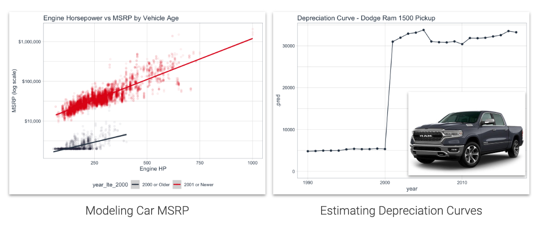
Estimate Depreciation Curves using Machine Learning
To implement the Depreciation Curve Estimation, you develop a machine learning model that is hyperparameter tuned using a 3-Stage Nested Hyper Parameter Tuning Process with 5-Fold Cross-Validation.
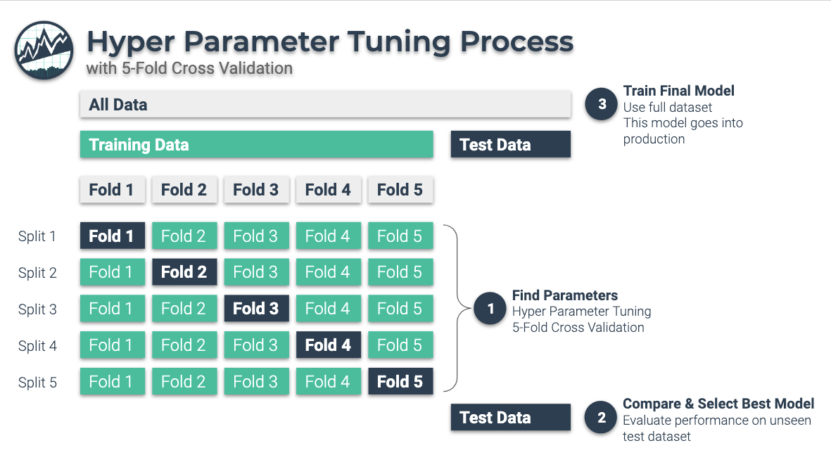
3-Stage Nested Hyperparameter Tuning Process
3 Stage Hyperparameter Tuning Process:
-
Find Parameters: Use Hyper Parameter Tuning on a “Training Dataset” that sections your training data into 5-Folds. The output at Stage 1 is the parameter set.
-
Compare and Select Best Model: Evaluate the performance on a hidden “Test Dataset”. The ouput at Stage 2 is that we determine best model.
-
Train Final Model: Once we have selected the best model, we train on the full dataset. This model goes into production.
Need to learn Data Science for Business? This is an advanced tutorial, but you can get the foundational skills, advanced machine learning, business consulting, and web application development using R, Shiny (Apps), H2O (ML), AWS (Cloud), and tidyverse (data manipulation and visualization). I recommend my 4-Course R-Track for Business Bundle.
Why Product Pricing is Important
Product price prediction is an important tool for businesses. There are key pricing actions that machine learning and algorithmic price modeling can be used for.

Which brands will customers pay more for?
Defend against inconsistent pricing
There is nothing more confusing to customers than pricing products inconsistently. Price too high, and customers fail to see the difference between competitor products and yours. Price too low and profit can suffer. Use machine learning to price products consistently based on the key product features that your customers care about.
Learn which features drive pricing and customer purchase decisions
In competitive markets, pricing is based on supply and demand economics. Sellers adjust prices to maximize profitability given market conditions. Use machine learning and explainable ML techniques to interpret the value of features such as brand (luxury vs economy), performance (engine horsepower), age (vehicle year), and more.
Develop price profiles (Appreciation / Depreciation Curves)
Another important concept to products like homes and automobiles is the ability to monitor the effect of time. Homes tend to appreciate and machinery (including automobiles) tend to depreciate in value over time. Use machine learning to develop price curves. We’ll do just that in this tutorial examining the MSRP of vehicles that were manufactured across time.
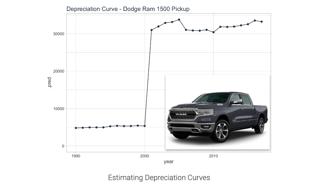
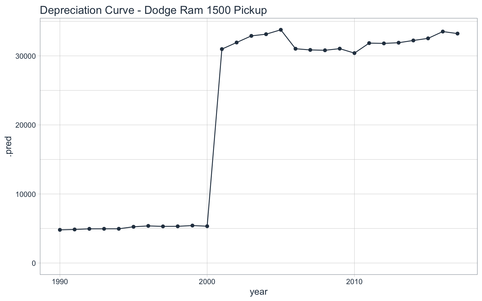
Depreciation Curve for Dodge Ram 1500 Pickup
Read on to learn how to make this plot
Product Price Tutorial
Onward - To the Product Price Prediction and Hyperparameter Tuning Tutorial.
1.0 Libraries and Data
Load the following libraries.
# Tidymodels
library(tune)
library(dials)
library(parsnip)
library(rsample)
library(recipes)
library(textrecipes)
library(yardstick)
library(vip)

# Parallel Processing
library(doParallel)
all_cores <- parallel::detectCores(logical = FALSE)
registerDoParallel(cores = all_cores)

# Data Cleaning
library(janitor)

# EDA
library(skimr)
library(correlationfunnel)
library(DataExplorer)

# ggplot2 Helpers
library(gghighlight)
library(patchwork)

# Core
library(tidyverse)
library(tidyquant)
library(knitr)
Next, get the data used for this tutorial. This data set containing Car Features and MSRP was scraped from "Edmunds and Twitter".

Download the Dataset
Car Features and MSRP Dataset
2.0 Data Understanding
Read the data using read_csv() and use clean_names() from the janitor package to clean up the column names.
car_prices_tbl <- read_csv("2020-01-21-tune/data/data.csv") %>%
    clean_names() %>%
    select(msrp, everything())

car_prices_tbl %>%
    head(5) %>%
    kable()
| msrp |
make |
model |
year |
engine_fuel_type |
engine_hp |
engine_cylinders |
transmission_type |
driven_wheels |
number_of_doors |
market_category |
vehicle_size |
vehicle_style |
highway_mpg |
city_mpg |
popularity |
| 46135 |
BMW |
1 Series M |
2011 |
premium unleaded (required) |
335 |
6 |
MANUAL |
rear wheel drive |
2 |
Factory Tuner,Luxury,High-Performance |
Compact |
Coupe |
26 |
19 |
3916 |
| 40650 |
BMW |
1 Series |
2011 |
premium unleaded (required) |
300 |
6 |
MANUAL |
rear wheel drive |
2 |
Luxury,Performance |
Compact |
Convertible |
28 |
19 |
3916 |
| 36350 |
BMW |
1 Series |
2011 |
premium unleaded (required) |
300 |
6 |
MANUAL |
rear wheel drive |
2 |
Luxury,High-Performance |
Compact |
Coupe |
28 |
20 |
3916 |
| 29450 |
BMW |
1 Series |
2011 |
premium unleaded (required) |
230 |
6 |
MANUAL |
rear wheel drive |
2 |
Luxury,Performance |
Compact |
Coupe |
28 |
18 |
3916 |
| 34500 |
BMW |
1 Series |
2011 |
premium unleaded (required) |
230 |
6 |
MANUAL |
rear wheel drive |
2 |
Luxury |
Compact |
Convertible |
28 |
18 |
3916 |
We can get a sense using some ggplot2 visualizations and correlation analysis to detect key features in the dataset.
2.1 Engine Horsepower vs MSRP
First, let’s take a look at two interesting factors to me:
- MSRP (vehicle price) - Our target, what customers on average pay for the vehicle, and
- Engine horsepower - A measure of product performance
car_plot_data_tbl <- car_prices_tbl %>%
    mutate(make_model = str_c(make, " ", model)) %>%
    select(msrp, engine_hp, make_model)

car_plot_data_tbl %>%
    ggplot(aes(engine_hp, msrp)) +
    geom_point(color = palette_light()["blue"], alpha = 0.15) +
    geom_smooth(method = "lm") +
    scale_y_log10(label = scales::dollar_format()) +
    theme_tq() +
    labs(title = "Engine Horsepower vs MSRP by Vehicle Age",
         x = "Engine HP", y = "MSRP (log scale)")
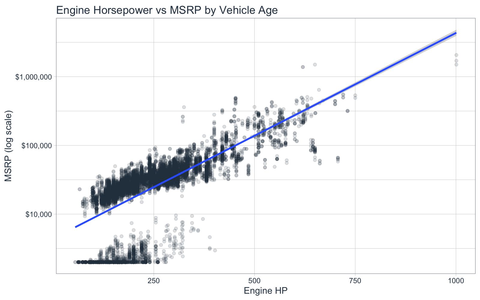
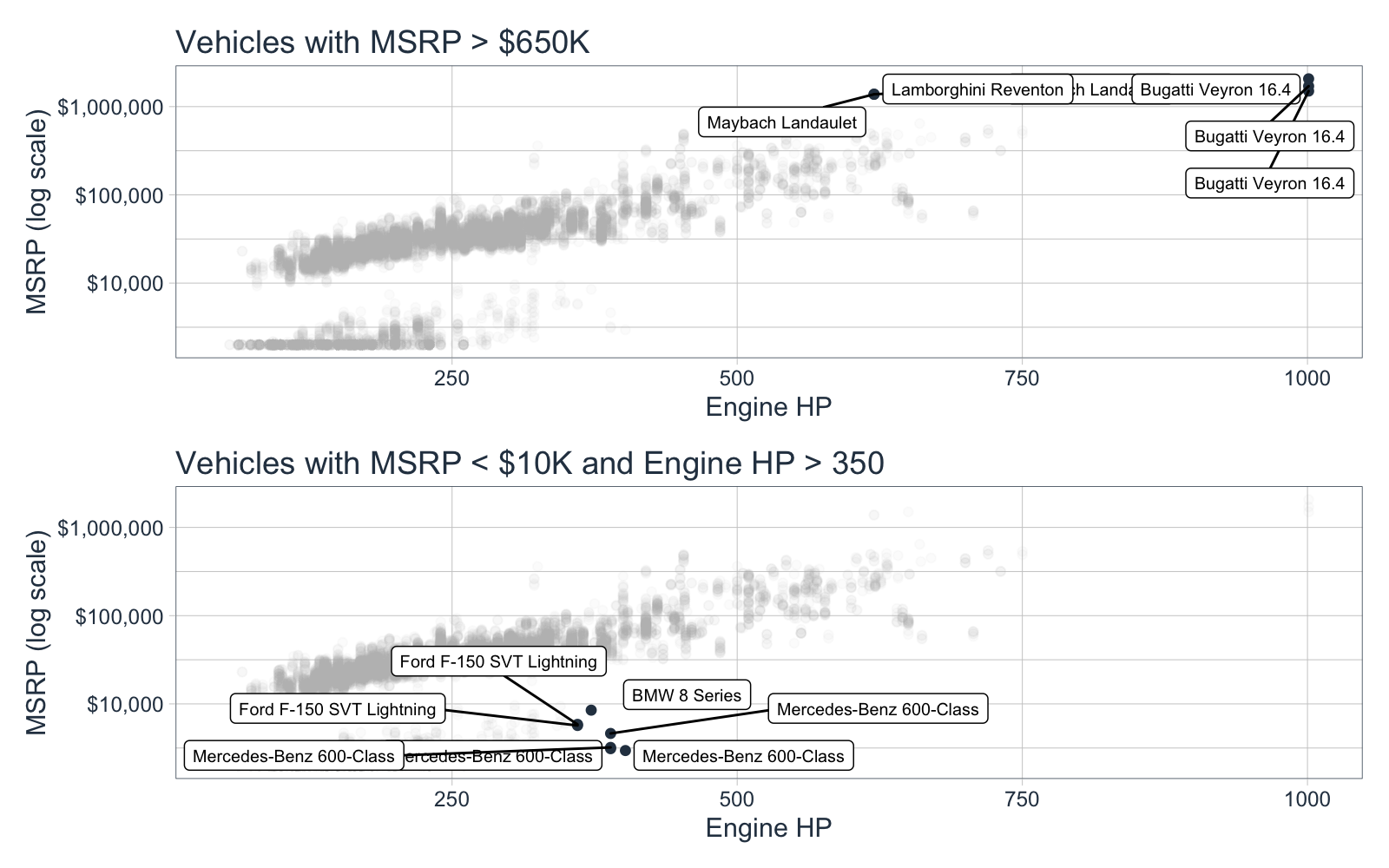
We can see that there are two distinct groups in the plots. We can inspect a bit closer with gghighlight and patchwork. I specifically focus on the high end of both groups:
- Vehicles with MSRP greater than $650,000
- Vehicles with Engine HP greater than 350 and MSRP less than $10,000
p1 <- car_plot_data_tbl %>%
    ggplot(aes(engine_hp, msrp)) +
    geom_point(color = palette_light()["blue"]) +
    scale_y_log10(label = scales::dollar_format()) +
    gghighlight(msrp > 650000, label_key = make_model,
                unhighlighted_colour = alpha("grey", 0.05),
                label_params = list(size = 2.5)) +
    theme_tq() +
    labs(title = "Vehicles with MSRP > $650K",
         x = "Engine HP", y = "MSRP (log scale)")

p2 <- car_plot_data_tbl %>%
    ggplot(aes(engine_hp, msrp)) +
    geom_point(color = palette_light()["blue"]) +
    scale_y_log10(label = scales::dollar_format()) +
    gghighlight(msrp < 10000, engine_hp > 350, label_key = make_model,
                unhighlighted_colour = alpha("grey", 0.05),
                label_params = list(size = 2.5), ) +
    theme_tq() +
    labs(title = "Vehicles with MSRP < $10K and Engine HP > 350",
         x = "Engine HP", y = "MSRP (log scale)")

# Patchwork for stacking ggplots on top of each other
p1 / p2
Key Points:
- The first group makes total sense - Lamborghini, Bugatti and Maybach. These are all super-luxury vehicles.
- The second group is more interesting - It’s BMW 8 Series, Mercedes-Benz 600-Class. This is odd to me because these vehicles normally have a higher starting price.
2.2 Correlation Analysis - correlationfunnel
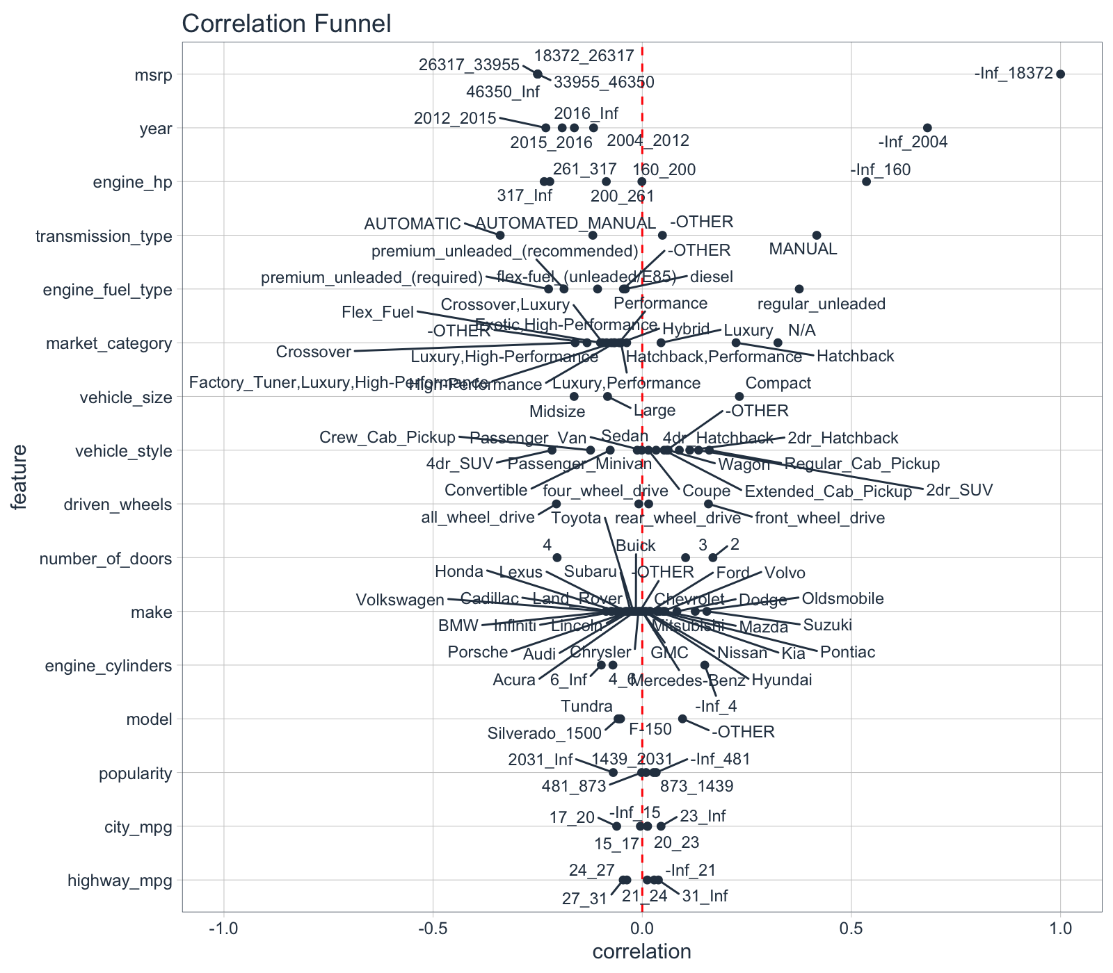
Next, I’ll use my correlationfunnel package to hone in on the low price vehicles. I want to find which features correlate most with low prices.
# correlationfunnel 3-step process
car_prices_tbl %>%
    drop_na(engine_hp, engine_cylinders, number_of_doors, engine_fuel_type) %>%
    binarize(n_bins = 5) %>%
    correlate(`msrp__-Inf_18372`) %>%
    plot_correlation_funnel()
Key Points:
Ah hah! The reduction in price is related to vehicle age. We can see that Vehicle Year less than 2004 is highly correlated with Vehicle Price (MSRP) less than $18,372. This explains why some of the 600 Series Mercedes-Benz vehicles (luxury brand) are in the low price group. Good - I’m not going crazy.
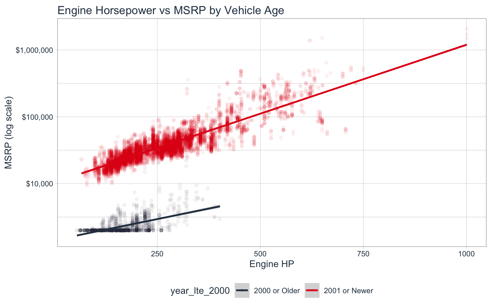
2.3 Engine HP, MSRP by Vehicle Age
Let’s explain this story by redo-ing the visualization from 2.1, this time segmenting by Vehicle Year. I’ll segment by year older than 2000 and newer than 2000.
car_plot_data_tbl <- car_prices_tbl %>%
    mutate(make_model = str_c(make, " ", model),
        year_lte_2000 = ifelse(year <= 2000, "2000 or Older", "2001 or Newer")
    ) %>%
    select(msrp, year_lte_2000, engine_hp, make_model)

car_plot_data_tbl %>%
    ggplot(aes(engine_hp, msrp, color = year_lte_2000)) +
    geom_point(alpha = 0.05) +
    scale_color_tq() +
    scale_y_log10(label = scales::dollar_format()) +
    geom_smooth(method = "lm") +
    theme_tq() +
    labs(title = "Engine Horsepower vs MSRP by Vehicle Age",
         x = "Engine HP", y = "MSRP (log scale)")
Key Points:
As Joshua Starmer would say, “Double Bam!” Vehicle Year is the culprit.
3.0 Exploratory Data Analysis
Ok, now that I have a sense of what is going on with the data, I need to figure out what’s needed to prepare the data for machine learning. The data set was webscraped. Datasets like this commonly have issues with missing data, unformatted data, lack of cleanliness, and need a lot of preprocessing to get into the format needed for modeling. We’ll fix that up with a preprocessing pipeline.
Goal
Our goal in this section is to identify data issues that need to be corrected. We will then use this information to develop a preprocessing pipeline. We will make heavy use of skimr and DataExplorer, two EDA packages I highly recommend.
3.1 Data Summary - skimr
I’m using the skim() function to breakdown the data by data type so I can assess missing values, number of uniue categories, numeric value distributions, etc.
skim(car_prices_tbl)
## Skim summary statistics
##  n obs: 11914
##  n variables: 16
##
## ── Variable type:character ───────────────────────────────────────────────────────────────────────────────────────────────
##           variable missing complete     n min max empty n_unique
##      driven_wheels       0    11914 11914  15  17     0        4
##   engine_fuel_type       3    11911 11914   6  44     0       10
##               make       0    11914 11914   3  13     0       48
##    market_category       0    11914 11914   3  54     0       72
##              model       0    11914 11914   1  35     0      915
##  transmission_type       0    11914 11914   6  16     0        5
##       vehicle_size       0    11914 11914   5   7     0        3
##      vehicle_style       0    11914 11914   5  19     0       16
##
## ── Variable type:numeric ─────────────────────────────────────────────────────────────────────────────────────────────────
##          variable missing complete     n     mean       sd   p0   p25   p50
##          city_mpg       0    11914 11914    19.73     8.99    7    16    18
##  engine_cylinders      30    11884 11914     5.63     1.78    0     4     6
##         engine_hp      69    11845 11914   249.39   109.19   55   170   227
##       highway_mpg       0    11914 11914    26.64     8.86   12    22    26
##              msrp       0    11914 11914 40594.74 60109.1  2000 21000 29995
##   number_of_doors       6    11908 11914     3.44     0.88    2     2     4
##        popularity       0    11914 11914  1554.91  1441.86    2   549  1385
##              year       0    11914 11914  2010.38     7.58 1990  2007  2015
##       p75    p100     hist
##     22        137 ▇▂▁▁▁▁▁▁
##      6         16 ▁▇▇▃▁▁▁▁
##    300       1001 ▅▇▃▁▁▁▁▁
##     30        354 ▇▁▁▁▁▁▁▁
##  42231.25 2065902 ▇▁▁▁▁▁▁▁
##      4          4 ▃▁▁▁▁▁▁▇
##   2009       5657 ▇▅▆▁▁▁▁▂
##   2016       2017 ▁▁▁▁▁▂▁▇
Key Points:
- We have missing values in a few features
- We have several categories with low and high unique values
- We have pretty high skew in several categories
Let’s go deeper with DataExplorer.
3.2 Missing Values - DataExplorer
Let’s use the plot_missing() function to identify which columns have missing values. We’ll take care of these missing values using imputation in section 4.
car_prices_tbl %>% plot_missing()
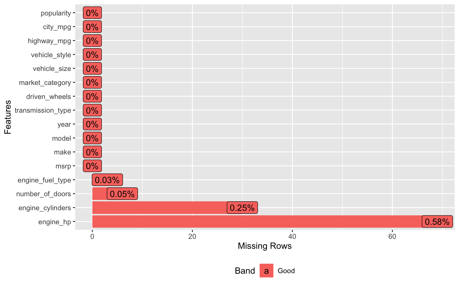
Key Point:
We’ll zap missing values and replace with estimated values using imputation.
3.3 Categorical Data - DataExplorer
Let’s use the plot_bar() function to identify the distribution of categories. We have several columns with a lot of categories that have few values. We can lump these into an “Other” Category.
car_prices_tbl %>% plot_bar(maxcat = 50, nrow = 2)
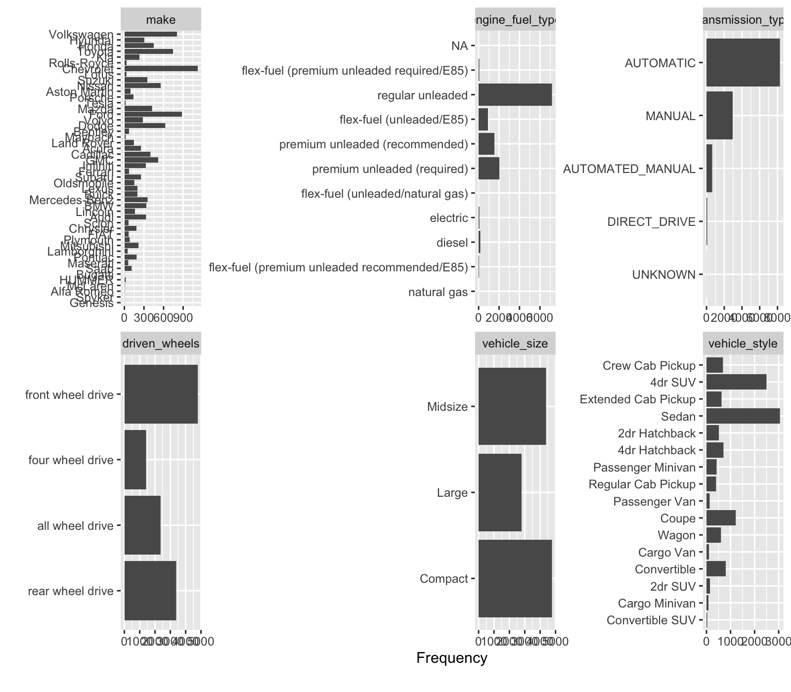
One category that doesn’t show up in the plot is “market_category”. This has 72 unique values - too many to plot. Let’s take a look.
car_prices_tbl %>% count(market_category, sort = TRUE)
## # A tibble: 72 x 2
##    market_category             n
##    <chr>                   <int>
##  1 N/A                      3742
##  2 Crossover                1110
##  3 Flex Fuel                 872
##  4 Luxury                    855
##  5 Luxury,Performance        673
##  6 Hatchback                 641
##  7 Performance               601
##  8 Crossover,Luxury          410
##  9 Luxury,High-Performance   334
## 10 Exotic,High-Performance   261
## # … with 62 more rows
Hmmm. This is actually a “tag”-style category (where one vehicle can have multiple tags). We can clean this up using term-frequency feature engineering.
Key Points:
- We need to lump categories with few observations
- We can use text-based feature engineering on the market categories that have multiple categories.
3.4 Numeric Data - DataExplorer
Let’s use plot_histogram() to investigate the numeric data. Some of these features are skewed and others are actually discrete (and best analyzed as categorical data). Skew won’t be much of an issue with tree-based algorithms so we’ll leave those alone (better from an explainability perspective). Discrete features like engine-cylinders and number of doors are better represented as factors.
car_prices_tbl %>% plot_histogram()
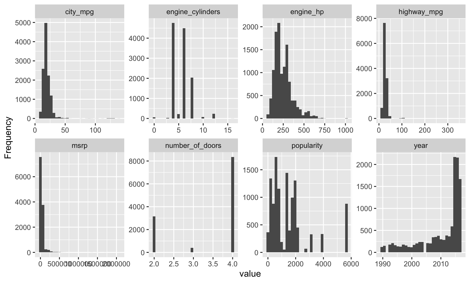
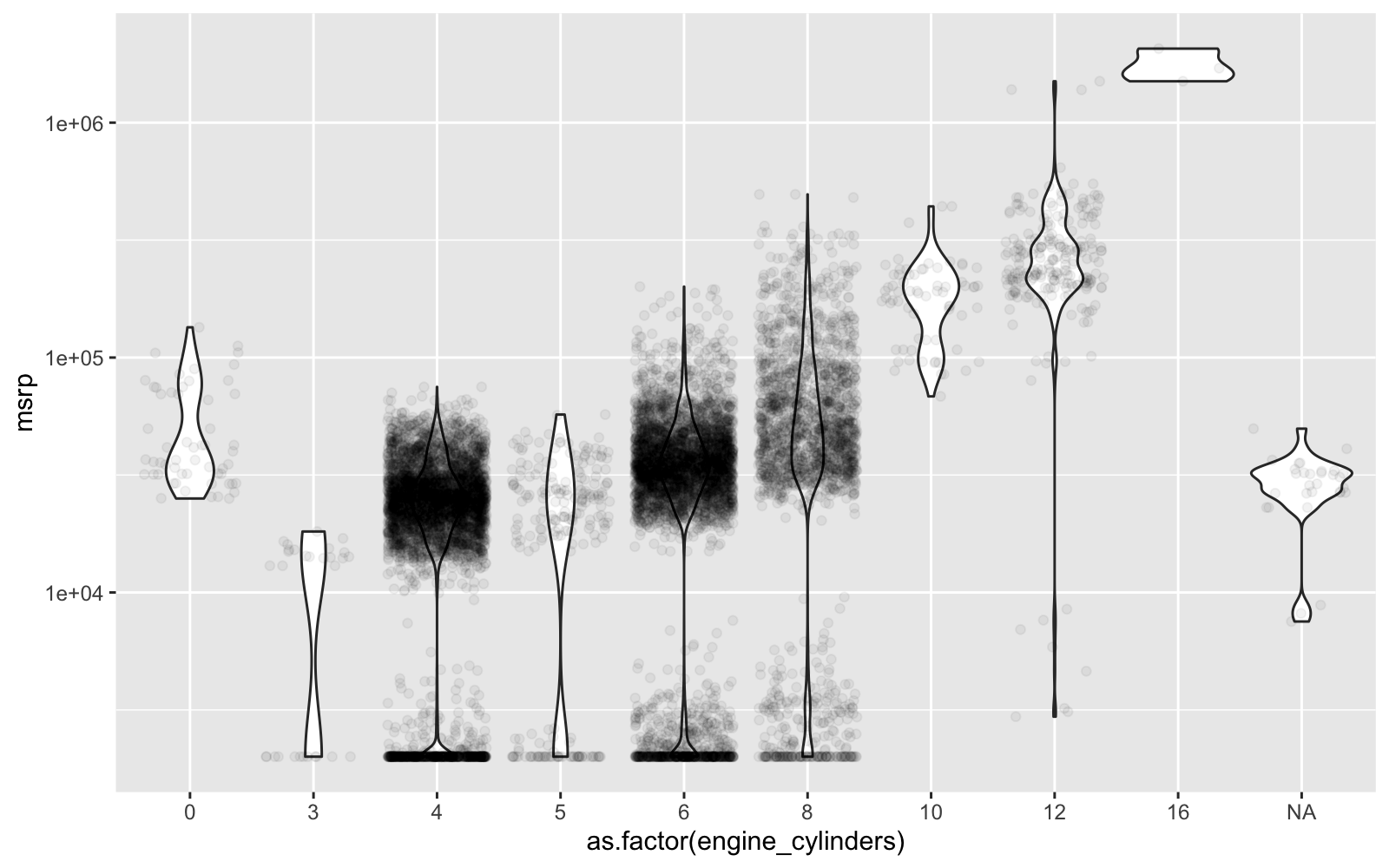
Here’s a closer look at engine cylinders vs MSRP. Definitely need to encode this one as a factor, which will be better because of the non-linear relationship to price. Note that cars with zero engine cylinders are electric.
car_prices_tbl %>%
    ggplot(aes(as.factor(engine_cylinders), msrp)) +
    geom_violin() +
    geom_jitter(alpha = 0.05) +
    scale_y_log10()
Key Points:
- We’ll encode engine cylinders and number of doors as categorical data to better represent non-linearity
- Tree-Based algorithms can handle skew. I’ll leave alone for explainability purposes. Note that you can use transformations like Box Cox to reduce skew for linear algorithms. But this transformation makes it more difficult to explain the results to non-technical stakeholders.
4.0 Machine Learning Strategy
You’re probably thinking, “Wow - That’s a lot of work just to get to this step.”
Yes, you’re right. That’s why good Data Scientists are in high demand. Data Scientists that understand business, know data wrangling, visualization techniques, can identify how to treat data prior to Machine Learning, and communicate what’s going on to the organization - These data scientists get good jobs.
At this point, it makes sense to re-iterate that I have a 4-Course R-Track Curriculum that will turn you into a good Data Scientist in 6-months or less. Yeahhhh!
ML Game Plan
We have a strategy that we are going to use to do what’s called “Nested Cross Validation”. It involves 3 Stages.

Stage 1: Find Parameters
We need to create several machine learning models and try them out. To accomplish we do:
- Initial Splitting - Separate into random training and test data sets
- Preprocessing - Make a pipeline to turn raw data into a dataset ready for ML
- Cross Validation Specification - Sample the training data into 5-splits
- Model Specification - Select model algorithms and identify key tuning parameters
- Grid Specification - Set up a grid using wise parameter choices
- Hyperparameter Tuning - Implement the tuning process
Stage 2: Select Best Model
Once we have the optimal algorithm parameters for each machine learning algorithm, we can move into stage 2. Our goal here is to compare each of the models on “Test Data”, data that were not used during the parameter tuning process. We re-train on the “Training Dataset” then evaluate against the “Test Dataset”. The best model has the best accuracy on this unseen data.
Stage 3: Retrain on the Full Dataset
Once we have the best model identified from Stage 2, we retrain the model using the best parameters from Stage 1 on the entire dataset. This gives us the best model to go into production with.
Ok, let’s get going.
5.0 Stage 1 - Preprocessing, Cross Validation, and Tuning
Time for machine learning! Just a few more steps and we’ll make and tune high-accuracy models.
5.1 Initial Train-Test Split - rsample
The first step is to split the data into Training and Testing sets. We use an 80/20 random split with the initial_split() function from rsample. The set.seed() function is used for reproducibility. Note that we have 11,914 cars (observations) of which 9,532 are randomly assigned to training and 2,382 are randomly assigned to testing.
set.seed(123)
car_initial_split <- initial_split(car_prices_tbl, prop = 0.80)
car_initial_split
## <9532/2382/11914>
5.2 Preprocessing Pipeline - recipes
What the heck is a preprocessing pipeline? A “preprocessing pipeline” (aka a “recipe”) is a set of preprocessing steps that transform raw data into data formatted for machine learning. The key advantage to a preprocessing pipeline is that it can be re-used on new data. So when you go into production, you can use the recipe to process new incoming data.
Remember in Section 3.0 when we used EDA to identify issues with our data? Now it’s time to fix those data issues using the Training Data Set. We use the recipe() function from the recipes package then progressively add step_* functions to transform the data.
The recipe we implement applies the following transformations:
- Encoding Character and Discrete Numeric data to Categorical Data.
- Text-Based Term Frequency Feature Engineering for the Market Category column
- Consolidate low-frequency categories
- Impute missing data using K-Nearest Neighbors with 5-neighbors (kNN is a fast and accurate imputation method)
- Remove unnecessary columns (e.g. model)
preprocessing_recipe <- recipe(msrp ~ ., data = training(car_initial_split)) %>%

    # Encode Categorical Data Types
    step_string2factor(all_nominal()) %>%
    step_mutate(
        engine_cylinders = as.factor(engine_cylinders),
        number_of_doors  = as.factor(number_of_doors)
    ) %>%

    # Feature Engineering - Market Category
    step_mutate(market_category = market_category %>% str_replace_all("_", "")) %>%
    step_tokenize(market_category) %>%
    step_tokenfilter(market_category, min_times = 0.05, max_times = 1, percentage = TRUE) %>%
    step_tf(market_category, weight_scheme = "binary") %>%

    # Combine low-frequency categories
    step_other(all_nominal(), threshold = 0.02, other = "other") %>%

    # Impute missing
    step_knnimpute(engine_fuel_type, engine_hp, engine_cylinders, number_of_doors,
                   neighbors = 5) %>%

    # Remove unnecessary columns
    step_rm(model) %>%
    prep()

preprocessing_recipe
## Data Recipe
##
## Inputs:
##
##       role #variables
##    outcome          1
##  predictor         15
##
## Training data contained 9532 data points and 84 incomplete rows.
##
## Operations:
##
## Factor variables from make, model, ... [trained]
## Variable mutation for  engine_cylinders, number_of_doors [trained]
## Variable mutation for  market_category [trained]
## Tokenization for market_category [trained]
## Text filtering for market_category [trained]
## Term frequency with market_category [trained]
## Collapsing factor levels for make, model, engine_fuel_type, ... [trained]
## K-nearest neighbor imputation for make, model, year, engine_hp, ... [trained]
## Variables removed model [trained]
The preprocessing recipe hasn’t yet changed the data. We’ve just come up with the recipe. To transform the data, we use bake(). I create a new variable to hold the preprocessed training dataset.
car_training_preprocessed_tbl <- preprocessing_recipe %>% bake(training(car_initial_split))
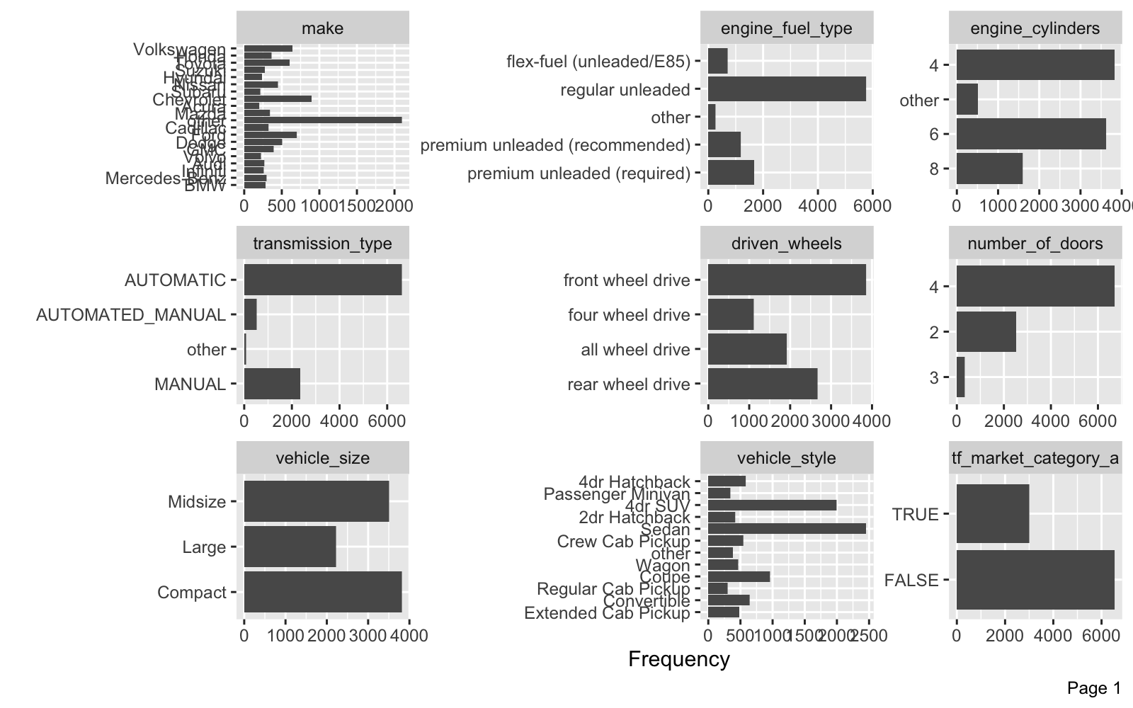
We can use DataExplorer to verify that the dataset has been processed. First, let’s inspect the Categorical Features.
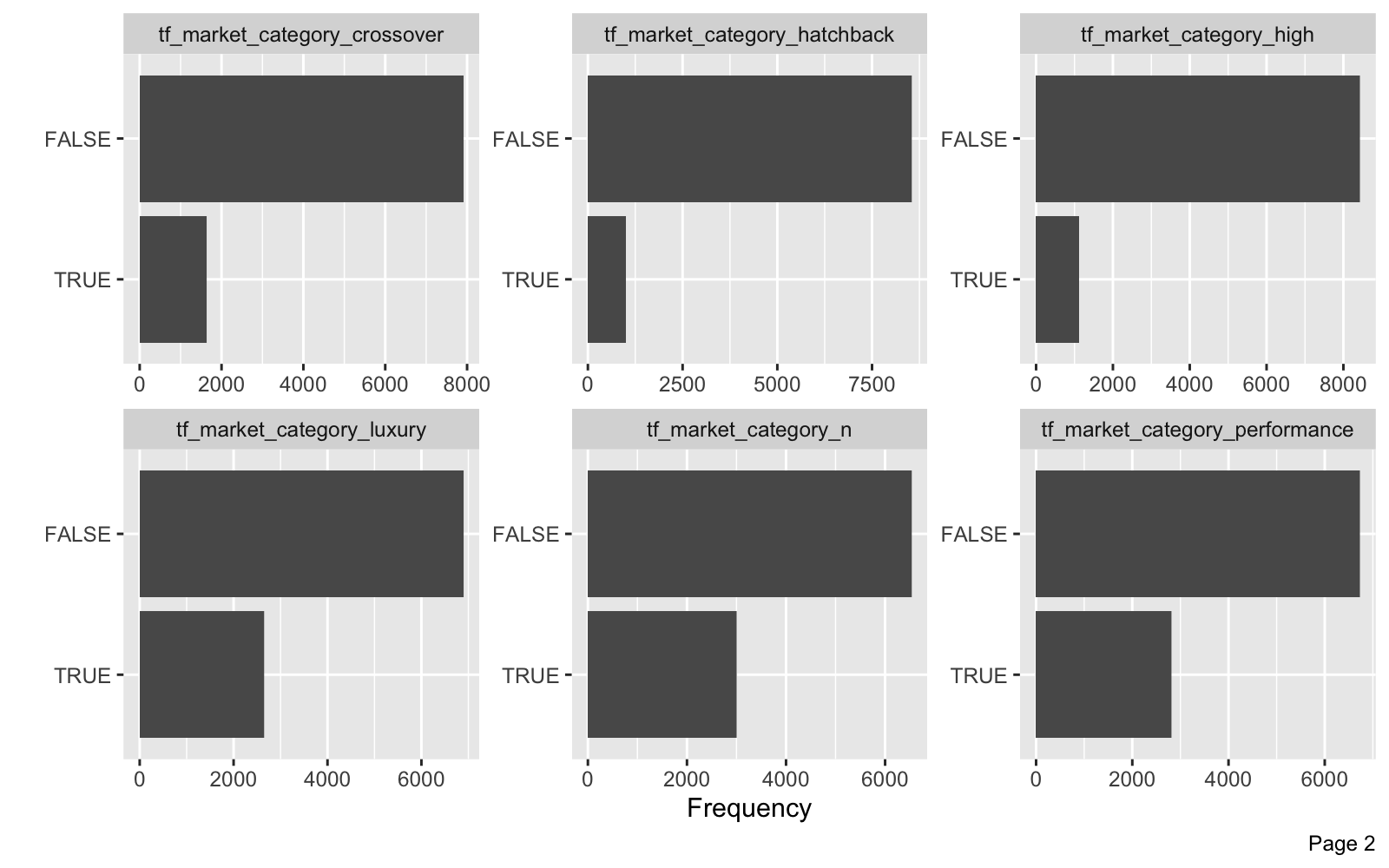
- The category distributions have been fixed - now “other” category present lumping together infrequent categories.
- The text feature processing has added several new columns beginning with “tf_market_category_”.
- Number of doors and engine cylinders are now categorical.
car_training_preprocessed_tbl %>% plot_bar(maxcat = 50)
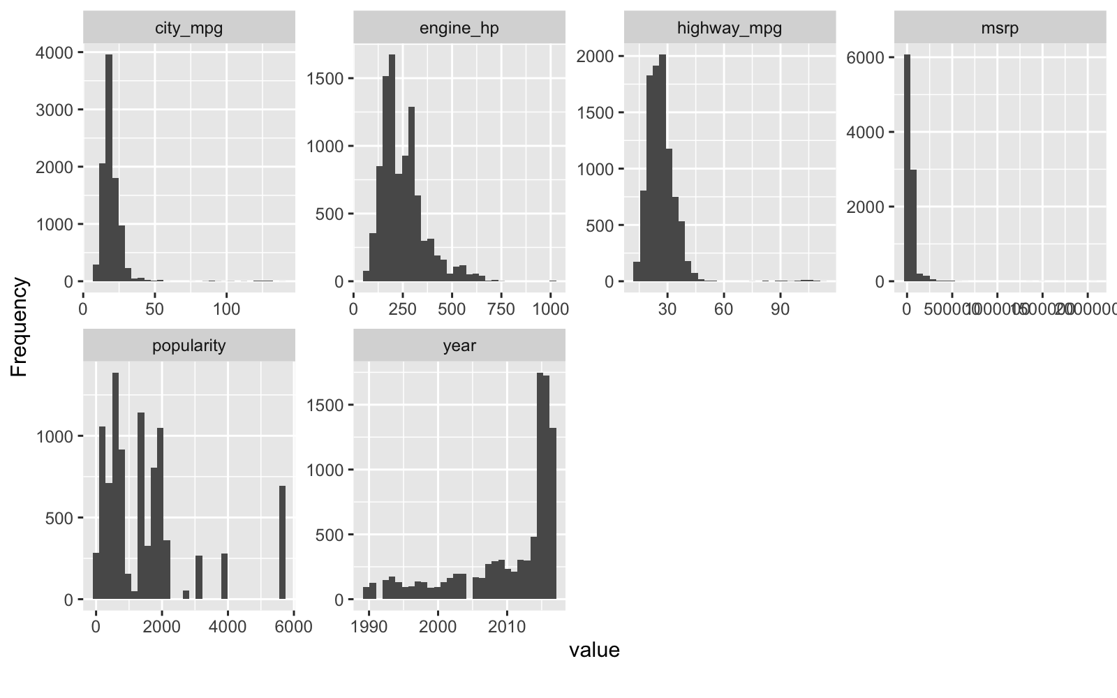
We can review the Numeric Features. The remaining numeric features have been left alone to preserve explainability.
car_training_preprocessed_tbl %>% plot_histogram()
5.3 Cross Validation Specification - rsample
Now that we have a preprocessing recipe and the initial training / testing split, we can develop the Cross Validation Specification. Standard practice is to use either a 5-Fold or 10-Fold cross validation:
- 5-Fold: I prefer 5-fold cross validation to speed up results by using 5 folds and an 80/20 split in each fold
- 10-Fold: Others prefer a 10-fold cross validation to use more training data with a 90/10 split in each fold. The downside is that this calculation requires twice as many models as 5-fold, which is already an expensive (time consuming) operation.
To implement 5-Fold Cross Validation, we use vfold_cv() from the rsample package. Make sure to use your training dataset (training()) and then apply the preprocessing recipe using bake() before the vfold_cv() cross validation sampling. You now have specified the 5-Fold Cross Validation specification for your training dataset.
set.seed(123)
car_cv_folds <- training(car_initial_split) %>%
    bake(preprocessing_recipe, new_data = .) %>%
    vfold_cv(v = 5)

car_cv_folds
## #  5-fold cross-validation
## # A tibble: 5 x 2
##   splits              id
##   <named list>        <chr>
## 1 <split [7.6K/1.9K]> Fold1
## 2 <split [7.6K/1.9K]> Fold2
## 3 <split [7.6K/1.9K]> Fold3
## 4 <split [7.6K/1.9K]> Fold4
## 5 <split [7.6K/1.9K]> Fold5
5.4 Model Specifications - parnsip
We’ll specify two competing models:
-
glmnet - Uses an Elastic Net, that combines the LASSO and Ridge Regression techniques. This is a linear algorithm, which can have difficulty with skewed numeric data, which is present in our numeric features.
-
xgboost - A tree-based algorithm that uses gradient boosted trees to develop high-performance models. The tree-based algorithms are not sensitive to skewed numeric data, which can easily be sectioned by the tree-splitting process.
5.4.1 glmnet - Model Spec
We use the linear_reg() function from parsnip to set up the initial specification. We use the tune() function from tune to identify the tuning parameters. We use set_engine() from parsnip to specify the engine as the glmnet library.
glmnet_model <- linear_reg(
        mode    = "regression",
        penalty = tune(),
        mixture = tune()
    ) %>%
    set_engine("glmnet")

glmnet_model
## Linear Regression Model Specification (regression)
##
## Main Arguments:
##   penalty = tune()
##   mixture = tune()
##
## Computational engine: glmnet
5.4.2 xgboost - Model Spec
A similar process is used for the XGBoost model. We specify boost_tree() and identify the tuning parameters. We set the engine to xgboost library. Note that an update to the xgboost library has changed the default objective from reg:linear to reg:squarederror. I’m specifying this by adding a objective argument in set_engine() that get’s passed to the underlying xgb.train(params = list([goes here])).
xgboost_model <- boost_tree(
        mode       = "regression",
        trees      = 1000,
        min_n      = tune(),
        tree_depth = tune(),
        learn_rate = tune()
    ) %>%
    set_engine("xgboost", objective = "reg:squarederror")

xgboost_model
## Boosted Tree Model Specification (regression)
##
## Main Arguments:
##   trees = 1000
##   min_n = tune()
##   tree_depth = tune()
##   learn_rate = tune()
##
## Engine-Specific Arguments:
##   objective = reg:squarederror
##
## Computational engine: xgboost
5.5 Grid Specification - dials
Next, we need to set up the grid that we plan to use for Grid Search. Grid Search is the process of specifying a variety of parameter values to be used with your model. The goal is to to find which combination of parameters yields the best accuracy (lowest prediction error) for each model.
We use the dials package to setup the hyperparameters. Key functions:
parameters() - Used to specify ranges for the tuning parametersgrid_*** - Grid functions including max entropy, hypercube, etc
5.5.1 glmnet - Grid Spec
For the glmnet model, we specify a parameter set, parameters(), that includes penalty() and mixture().
glmnet_params <- parameters(penalty(), mixture())
glmnet_params
## Collection of 2 parameters for tuning
##
##       id parameter type object class
##  penalty        penalty    nparam[+]
##  mixture        mixture    nparam[+]
Next, we use the grid_max_entropy() function to make a grid of 20 values using the parameters. I use set.seed() to make this random process reproducible.
set.seed(123)
glmnet_grid <- grid_max_entropy(glmnet_params, size = 20)
glmnet_grid
## # A tibble: 20 x 2
##     penalty mixture
##       <dbl>   <dbl>
##  1 2.94e- 1  0.702
##  2 1.48e- 4  0.996
##  3 1.60e- 1  0.444
##  4 5.86e- 1  0.975
##  5 1.69e- 9  0.0491
##  6 1.10e- 5  0.699
##  7 2.76e- 2  0.988
##  8 4.95e- 8  0.753
##  9 1.07e- 5  0.382
## 10 7.87e- 8  0.331
## 11 4.07e- 1  0.180
## 12 1.70e- 3  0.590
## 13 2.52e-10  0.382
## 14 2.47e-10  0.666
## 15 2.31e- 9  0.921
## 16 1.31e- 7  0.546
## 17 1.49e- 6  0.973
## 18 1.28e- 3  0.0224
## 19 7.49e- 7  0.0747
## 20 2.37e- 3  0.351
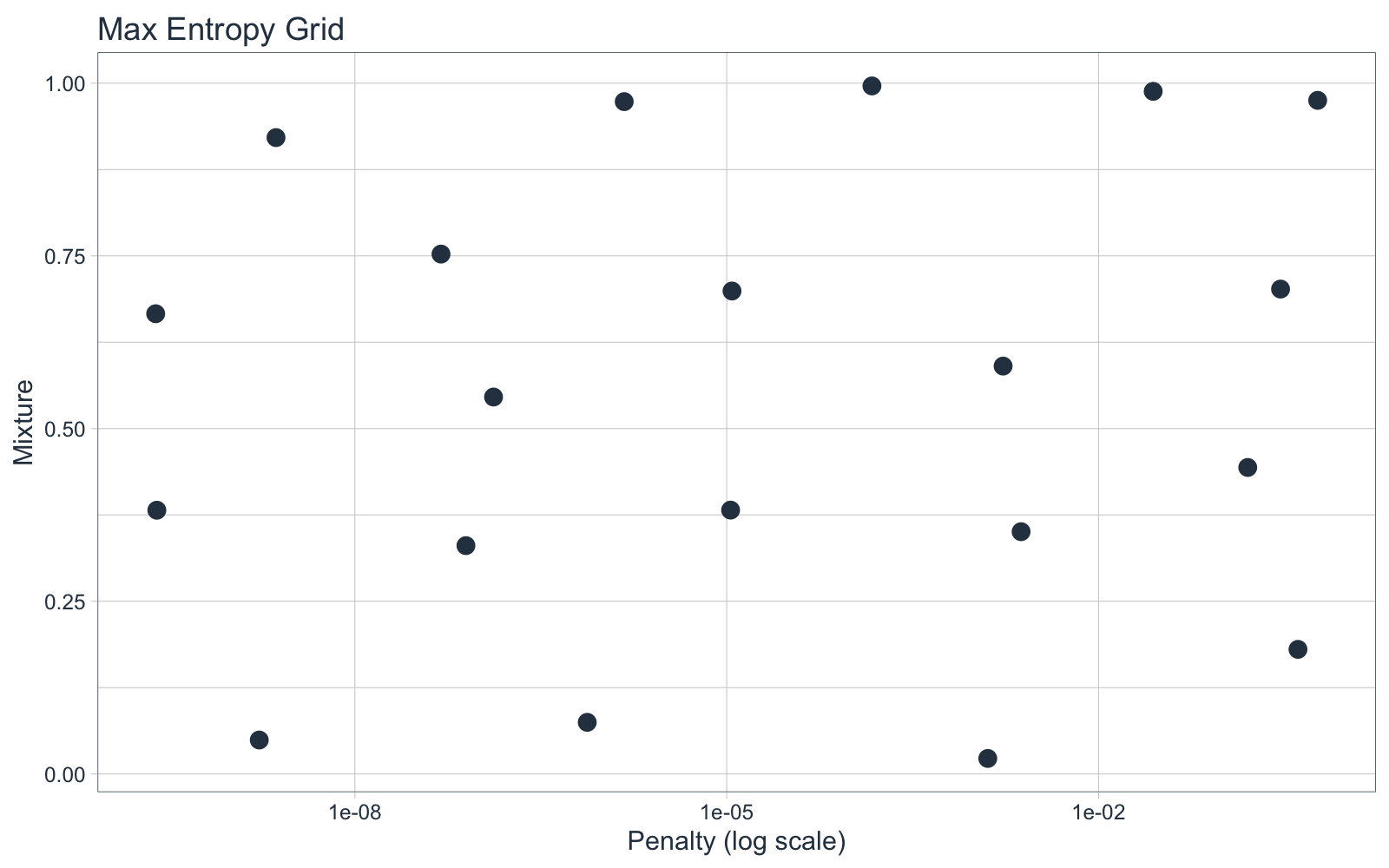
Because this is a 2-Dimensional Hyper Paramater Space (only 2 tuning parameters), we can visualize what the grid_max_entropy() function did. The grid selections were evenly spaced out to create uniformly distributed hyperparameter selections. Note that the penalty parameter is on the Log Base 10-scale by default (refer to the dials::penalty() function documentation). This functionality results in smarter choices for critical parameters, a big benefit of using the tidymodels framework.
glmnet_grid %>%
    ggplot(aes(penalty, mixture)) +
    geom_point(color = palette_light()["blue"], size = 3) +
    scale_x_log10() +
    theme_tq() +
    labs(title = "Max Entropy Grid", x = "Penalty (log scale)", y = "Mixture")
5.5.2 xgboost - Grid Spec
We can follow the same process for the xgboost model, specifying a parameter set using parameters(). The tuning parameters we select for are grid are made super easy using the min_n(), tree_depth(), and learn_rate() functions from dials().
xgboost_params <- parameters(min_n(), tree_depth(), learn_rate())
xgboost_params
## Collection of 3 parameters for tuning
##
##          id parameter type object class
##       min_n          min_n    nparam[+]
##  tree_depth     tree_depth    nparam[+]
##  learn_rate     learn_rate    nparam[+]
Next, we set up the grid space. Because this is now a 3-Dimensional Hyperparameter Space, I up the size of the grid to 30 points. Note that this will drastically increase the time it takes to tune the models because the xgboost algorithm must be run 30 x 5 = 150 times. Each time it runs with 1000 trees, so we are talking 150,000 tree calculations. My point is that it will take a bit to run the algorithm once we get to Section 5.6 Hyperparameter Tuning.
set.seed(123)
xgboost_grid <- grid_max_entropy(xgboost_params, size = 30)
xgboost_grid
## # A tibble: 30 x 3
##    min_n tree_depth    learn_rate
##    <int>      <int>         <dbl>
##  1    39          1 0.00000106
##  2    37          9 0.000749
##  3     2          9 0.0662
##  4    27          9 0.00000585
##  5     5         14 0.00000000259
##  6    17          2 0.000413
##  7    34         11 0.0000000522
##  8    10          4 0.0856
##  9    28          3 0.000000156
## 10    24          8 0.00159
## # … with 20 more rows
5.6 Hyper Parameter Tuning - tune
Now that we have specified the recipe, models, cross validation spec, and grid spec, we can use tune() to bring them all together to implement the Hyperparameter Tuning with 5-Fold Cross Validation.
5.6.1 glmnet - Hyperparameter Tuning
Tuning the model using 5-fold Cross Validation is straight-forward with the tune_grid() function. We specify the formula, model, resamples, grid, and metrics.
The only piece that I haven’t explained is the metrics. These come from the yardstick package, which has functions including mae(), mape(), rsme() and rsq() for calculating regression accuracy. We can specify any number of these using the metric_set(). Just make sure to use only regression metrics since this is a regression problem. For classification, you can use all of the normal measures like AUC, Precision, Recall, F1, etc.
glmnet_stage_1_cv_results_tbl <- tune_grid(
    formula   = msrp ~ .,
    model     = glmnet_model,
    resamples = car_cv_folds,
    grid      = glmnet_grid,
    metrics   = metric_set(mae, mape, rmse, rsq),
    control   = control_grid(verbose = TRUE)
)
Use the show_best() function to quickly identify the best hyperparameter values.
glmnet_stage_1_cv_results_tbl %>% show_best("mae", n = 10, maximize = FALSE)
## # A tibble: 10 x 7
##     penalty mixture .metric .estimator   mean     n std_err
##       <dbl>   <dbl> <chr>   <chr>       <dbl> <int>   <dbl>
##  1 1.28e- 3  0.0224 mae     standard   16801.     5    117.
##  2 1.69e- 9  0.0491 mae     standard   16883.     5    114.
##  3 7.49e- 7  0.0747 mae     standard   16891.     5    112.
##  4 4.07e- 1  0.180  mae     standard   16898.     5    111.
##  5 7.87e- 8  0.331  mae     standard   16910.     5    110.
##  6 2.37e- 3  0.351  mae     standard   16910.     5    110.
##  7 1.07e- 5  0.382  mae     standard   16911.     5    110.
##  8 2.52e-10  0.382  mae     standard   16911.     5    110.
##  9 1.60e- 1  0.444  mae     standard   16912.     5    111.
## 10 1.31e- 7  0.546  mae     standard   16914.     5    113.
Key Point:
A key observation is that the Mean Absolute Error (MAE) is $16,801, meaning the model is performing poorly. This is partly because we left the numeric features untransformed. Try updating the recipe with step_boxcox() and see if you can do better. Note that your MSRP will be transformed so you need to invert the MAE to the correct scale by finding the power for the box-cox transformation. But I digress.
5.6.2 xgboost - Hyperparameter Tuning
Follow the same tuning process for the xgboost model using tune_grid().
Warning: This takes approximately 20 minutes to run with 6-core parallel backend. I have recommendations to speed up this at the end of the article.
xgboost_stage_1_cv_results_tbl <- tune_grid(
    formula   = msrp ~ .,
    model     = xgboost_model,
    resamples = car_cv_folds,
    grid      = xgboost_grid,
    metrics   = metric_set(mae, mape, rmse, rsq),
    control   = control_grid(verbose = TRUE)
)
We can see the best xgboost tuning parameters with show_best().
xgboost_stage_1_cv_results_tbl %>% show_best("mae", n = 10, maximize = FALSE)
## # A tibble: 10 x 8
##    min_n tree_depth learn_rate .metric .estimator   mean     n std_err
##    <int>      <int>      <dbl> <chr>   <chr>       <dbl> <int>   <dbl>
##  1     2          9   0.0662   mae     standard    3748.     5   151.
##  2     9         15   0.0117   mae     standard    4048.     5    44.1
##  3    21         12   0.0120   mae     standard    4558.     5    91.3
##  4    10          4   0.0856   mae     standard    4941.     5   113.
##  5    24          3   0.00745  mae     standard    7930.     5   178.
##  6    37          2   0.00547  mae     standard    9169.     5   210.
##  7    24          8   0.00159  mae     standard    9258.     5   347.
##  8    37          9   0.000749 mae     standard   19514.     5   430.
##  9     3          1   0.000476 mae     standard   27905.     5   377.
## 10    17          2   0.000413 mae     standard   28124.     5   385.
Key Point:
A key observation is that the Mean Absolute Error (MAE) is $3,784, meaning the xgboost model is performing about 5X better than the glmnet. However, we won’t know for sure until we move to Stage 2, Evaluation.
6.0 Stage 2 - Compare and Select Best Model
Feels like a whirlwind to get to this point. You’re doing great. Just a little bit more to go. Now, let’s compare our models.
The “proper” way to perform model selection is not to use the cross validation results because in theory we’ve optimized the results to the data the training data. This is why we left out the testing set by doing initial splitting at the beginning.
Now, do I agree with this? Let me just say that normally the Cross Validation Winner is the true winner.
But for the sake of showing you the correct way, I will continue with the model comparison.
6.1 Select the Best Parameters
Use the select_best() function from the tune package to get the best parameters. We’ll do this for both the glment and xgboost models.
params_glmnet_best <- glmnet_stage_1_cv_results_tbl %>%
    select_best("mae", maximize = FALSE)

params_glmnet_best
## # A tibble: 1 x 2
##   penalty mixture
##     <dbl>   <dbl>
## 1 0.00128  0.0224
params_xgboost_best <- xgboost_stage_1_cv_results_tbl %>%
    select_best("mae", maximize = FALSE)

params_xgboost_best
## # A tibble: 1 x 3
##   min_n tree_depth learn_rate
##   <int>      <int>      <dbl>
## 1     2          9     0.0662
6.2 Finalize the Models
Next, we can use the finalize_model() function to apply the best parameters to each of the models. Do this for both the glmnet and xgboost models.
glmnet_stage_2_model <- glmnet_model %>%
    finalize_model(parameters = params_glmnet_best)

glmnet_stage_2_model
## Linear Regression Model Specification (regression)
##
## Main Arguments:
##   penalty = 0.00127732582071729
##   mixture = 0.0224261444527656
##
## Computational engine: glmnet
xgboost_stage_2_model <- xgboost_model %>%
    finalize_model(params_xgboost_best)

xgboost_stage_2_model
## Boosted Tree Model Specification (regression)
##
## Main Arguments:
##   trees = 1000
##   min_n = 2
##   tree_depth = 9
##   learn_rate = 0.0661551553016808
##
## Engine-Specific Arguments:
##   objective = reg:squarederror
##
## Computational engine: xgboost
We can create a helper function, calc_test_metrics(), to calculate the performance on the test set.
calc_test_metrics <- function(formula, model_spec, recipe, split) {

    train_processed <- training(split) %>% bake(recipe, new_data = .)
    test_processed  <- testing(split) %>% bake(recipe, new_data = .)

    target_expr <- recipe %>%
        pluck("last_term_info") %>%
        filter(role == "outcome") %>%
        pull(variable) %>%
        sym()

    model_spec %>%
        fit(formula = as.formula(formula),
            data    = train_processed) %>%
        predict(new_data = test_processed) %>%
        bind_cols(testing(split)) %>%
        metrics(!! target_expr, .pred)
}
Use the calc_test_metrics() function to calculate the test performance on the glmnet model.
glmnet_stage_2_metrics <- calc_test_metrics(
    formula    = msrp ~ .,
    model_spec = glmnet_stage_2_model,
    recipe     = preprocessing_recipe,
    split      = car_initial_split
)
glmnet_stage_2_metrics
## # A tibble: 3 x 3
##   .metric .estimator .estimate
##   <chr>   <chr>          <dbl>
## 1 rmse    standard   36200.
## 2 rsq     standard       0.592
## 3 mae     standard   16593.
Use the calc_test_metrics() function to calculate the test performance on the xgboost model.
xgboost_stage_2_metrics <- calc_test_metrics(
    formula    = msrp ~ .,
    model_spec = xgboost_stage_2_model,
    recipe     = preprocessing_recipe,
    split      = car_initial_split
)
xgboost_stage_2_metrics
## # A tibble: 3 x 3
##   .metric .estimator .estimate
##   <chr>   <chr>          <dbl>
## 1 rmse    standard   11577.
## 2 rsq     standard       0.961
## 3 mae     standard    3209.
6.4 Model Winner!
Winner: The xgboost model had an MAE of $3,209 on the test data set. We select this model with the following parameters to move forward.
xgboost_stage_2_model
## Boosted Tree Model Specification (regression)
##
## Main Arguments:
##   trees = 1000
##   min_n = 2
##   tree_depth = 9
##   learn_rate = 0.0661551553016808
##
## Engine-Specific Arguments:
##   objective = reg:squarederror
##
## Computational engine: xgboost
7.0 Stage 3 - Final Model (Full Dataset)
Now that we have a winner from Stage 2, we move forward with the xgboost model and train on the full data set. This gives us the best possible model to move into production with.
Use the fit() function from parsnip to train the final xgboost model on the full data set. Make sure to apply the preprocessing recipe to the original car_prices_tbl.
model_final <- xgboost_stage_2_model %>%
    fit(msrp ~ . , data = bake(preprocessing_recipe, new_data = car_prices_tbl))
8.0 Making Predictions on New Data
We’ve went through the full analysis and have a “production-ready” model. Now for some fun - let’s use it on some new data. To avoid repetitive code, I created the helper function, predict_msrp(), to quickly apply my final model and preprocessing recipe to new data.
predict_msrp <- function(new_data,
                         model  = model_final,
                         recipe = preprocessing_recipe) {
    new_data %>%
        bake(recipe, new_data = .) %>%
        predict(model, new_data = .)
}
8.1 What does a
I’ll simulate a 2008 Dodge Ram 1500 Pickup and calculate the predicted price.
dodge_ram_tbl <- tibble(
    make = "Dodge",
    model = "Ram 1500 Pickup",
    year = 2008,
    engine_fuel_type = "regular unleaded",
    engine_hp = 300,
    engine_cylinders = 8,
    transmission_type = "AUTOMATIC",
    driven_wheels = "four wheel drive",
    number_of_doors = "2",
    market_category = "N/A",
    vehicle_size = "Compact",
    vehicle_style = "Extended Cab Pickup",
    highway_mpg = 19,
    city_mpg = 13,
    popularity = 1851
)

dodge_ram_tbl %>% predict_msrp()
## # A tibble: 1 x 1
##    .pred
##    <dbl>
## 1 30813.
8.2 What’s the “Luxury” Effect?
Let’s play with the model a bit. Next, let’s change the market_category from “N/A” to “Luxury”. The price just jumped from $30K to $50K.
luxury_dodge_ram_tbl <- tibble(
    make = "Dodge",
    model = "Ram 1500 Pickup",
    year = 2008,
    engine_fuel_type = "regular unleaded",
    engine_hp = 300,
    engine_cylinders = 8,
    transmission_type = "AUTOMATIC",
    driven_wheels = "four wheel drive",
    number_of_doors = "2",

    # Change from N/A to Luxury
    market_category = "Luxury",
    vehicle_size = "Compact",
    vehicle_style = "Extended Cab Pickup",
    highway_mpg = 19,
    city_mpg = 13,
    popularity = 1851
)

luxury_dodge_ram_tbl %>% predict_msrp()
## # A tibble: 1 x 1
##    .pred
##    <dbl>
## 1 49986.
8.3 How Do Prices Vary By Model Year?
Let’s see how our XGBoost model views the effect of changing the model year. First, we’ll create a dataframe of Dodge Ram 1500 Pickups with the only feature that changes is the model year.
dodge_rams_tbl <- tibble(year = 2017:1990) %>%
    bind_rows(dodge_ram_tbl) %>%
    fill(names(.), .direction = "up") %>%
    distinct()

dodge_rams_tbl
## # A tibble: 28 x 15
##     year make  model engine_fuel_type engine_hp engine_cylinders
##    <dbl> <chr> <chr> <chr>                <dbl>            <dbl>
##  1  2017 Dodge Ram … regular unleaded       300                8
##  2  2016 Dodge Ram … regular unleaded       300                8
##  3  2015 Dodge Ram … regular unleaded       300                8
##  4  2014 Dodge Ram … regular unleaded       300                8
##  5  2013 Dodge Ram … regular unleaded       300                8
##  6  2012 Dodge Ram … regular unleaded       300                8
##  7  2011 Dodge Ram … regular unleaded       300                8
##  8  2010 Dodge Ram … regular unleaded       300                8
##  9  2009 Dodge Ram … regular unleaded       300                8
## 10  2008 Dodge Ram … regular unleaded       300                8
## # … with 18 more rows, and 9 more variables: transmission_type <chr>,
## #   driven_wheels <chr>, number_of_doors <chr>, market_category <chr>,
## #   vehicle_size <chr>, vehicle_style <chr>, highway_mpg <dbl>, city_mpg <dbl>,
## #   popularity <dbl>
Next, we can use ggplot2 to visualize this “Year” effect, which is essentially a Depreciation Curve. We can see that there’s a huge depreciation going from models built in 1990’s vs 2000’s and earlier.
predict_msrp(dodge_rams_tbl) %>%
    bind_cols(dodge_rams_tbl) %>%
    ggplot(aes(year, .pred)) +
    geom_line(color = palette_light()["blue"]) +
    geom_point(color = palette_light()["blue"]) +
    expand_limits(y = 0) +
    theme_tq() +
    labs(title = "Depreciation Curve - Dodge Ram 1500 Pickup")
8.4 Which Features Are Most Important?
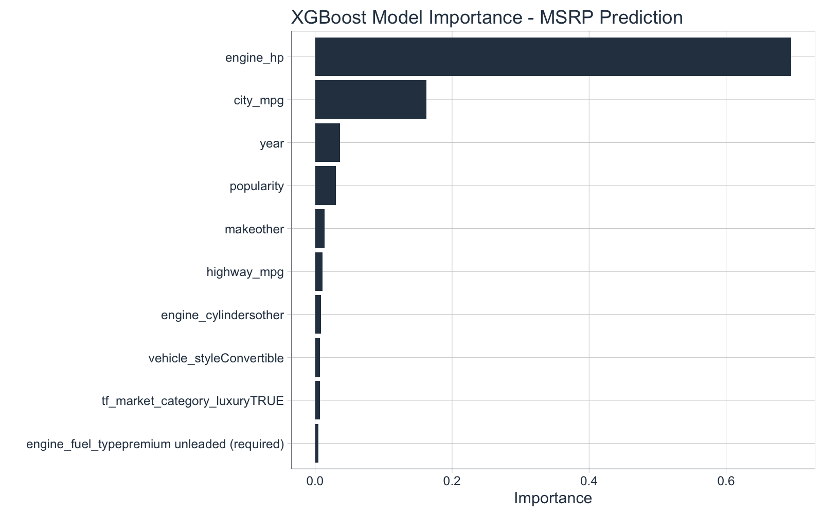
Finally, we can check which features have the most impact on the MSRP using the vip() function from the vip (variable importance) package.
vip(model_final, aesthetics = list(fill = palette_light()["blue"])) +
    labs(title = "XGBoost Model Importance - MSRP Prediction") +
    theme_tq()
9.0 Conclusion and Next Steps
The tune package presents a much needed tool for Hyperparameter Tuning in the tidymodels ecosystem. We saw how useful it was to perform 5-Fold Cross Validation, a standard in improving machine learning performance.
An advanced machine learning package that I’m a huge fan of is h2o. H2O provides a automatic machine learning, which takes a similar approach (minus the Stage 2 - Comparison Step) by automating the cross validation and hyperparameter tuning process. Because H2O is written in Java, H2O is much faster and more scalable, which is great for large-scale machine learning projects. If you are interested in learning h2o, I recommend my 4-Course R-Track for Business Program - The 201 Course teaches Advanced ML with H2O.
The last step is to productionalize the model inside a Shiny Web Application. I teach two courses on production with Shiny:
Shiny Dashboards - Build 2 Predictive Web DashboardsShiny Developer with AWS - Build Full-Stack Web Applications in the Cloud
The two Shiny courses are part of the 4-Course R-Track for Business Program.