DataExplorer: Exploratory Data Analysis in R
Written by Matt Dancho
Did you know that 80% of data science is spent cleaning & preparing data for analysis? Yep, that’s right! NOT modeling (the fun stuff). This process is called Exploratory Data Analysis (EDA). R has an excellent Exploratory Data Analysis solution that is almost guaranteed to speed up your exploratory analysis 10X: It’s called DataExplorer. And I’m going to get you up and running with DataExplorer in under 5-minutes. Here’s what you learn in this R-Tip:
- How to make an Automatic EDA Report in seconds with
DataExplorer
- BONUS: How to use the 7 most important EDA Plots to get exploratory insights.
R-Tips Weekly
This article is part of R-Tips Weekly, a weekly video tutorial that shows you step-by-step how to do common R coding tasks.
Here are the links to get set up. 👇
This Tutorial Is Available In Video
I have a companion video tutorial that shows even more secrets (plus mistakes to avoid). And, I’m finding that a lot of my students prefer the dialogue that goes along with coding. So check out this video to see me running the code in this tutorial. 👇
What Is Exploratory Data Analysis?
Exploratory Data Analysis (EDA) is how data scientists and data analysts find meaningful information in the form of relationships in the data. EDA is absolutely critical as a first step before machine learning and to explain business insights to non-technical stakeholders like executives and business leadership.
Make exploratory data analysis visuals with DataExplorer
What Do I Make In This R-Tip?
By the end of this R-Tip, you’ll make this exploratory data analysis report with 7 exploratory plots. Perfect for impressing your boss and coworkers! (Nice EDA skills)
Don't forget to get the code.
Thank You Developers.
Before we dive into DataExplorer, I want to take a moment to thank the developer, Boxuan Cui. He’s currently working as a Senior Data Science Manager at Tripadvisor. In his spare time, Boxuan has built and maintains one of the most useful R packages on the planet: DataExplorer. Thank you!
Exploratory Data Analysis with DataExplorer
One of the coolest features of DataExplorer is the ability to create an EDA Report in 1 line of code. This automates:
- Basic Statistics
- Data Structure
- Missing Data Profiling
- Continuous and Categorical Distribution Profiling (Histograms, Bar Charts)
- Relationships (Correlation)
Ultimately, this saves the analyst/data scientist SO MUCH TIME.
Step 1: Load the libraries and data
To get set up, all we need to do is load the following libraries and data.
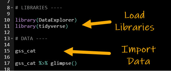
Get the code.
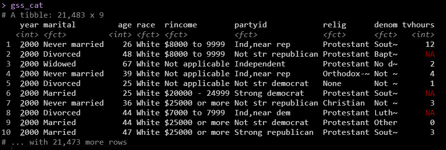
We’ll use the gss_cat dataset, which has income levels for people by various factors including marital status, age, race, religion, ….
With data in hand, we are ready to create the automatic EDA report. Let’s go!
Step 2: Create the EDA Report
Next, use create_report() to make our EDA report. Be sure to specify the output file, output directory, target variable (y), and give it a report title.
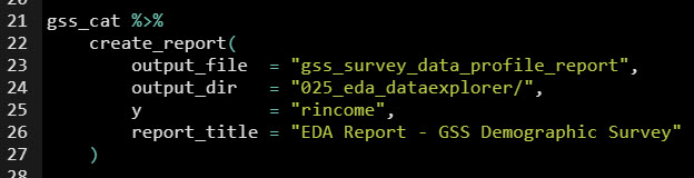
Get the code.
This produces an automatic EDA report that covers all of the important aspects that we need to analyze in our data! It’s that simple folks.
The report is great, but the next thing you’re probably wondering is how the heck am I going to use this report.
That’s why I want to show you…
BONUS: How to use the 7 Most Important DataExplorer Plots
As an extra special bonus, I figured I’d teach you not only how to make the report BUT how to use the report too. Here’s how to get the most out of your automatic EDA report. If you’d like to get the code to produce the individual plots, just sign up for my FREE R-tips codebase. You’ll get all the code sent to your email plus more R-Tips every week.
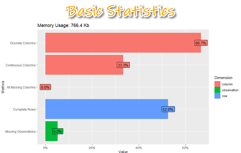
1. Basic Statistics
Get the code.
The basic statistics is where we first start understanding our data. We can see information about our columns including:
- Discrete columns: Columns with categorical data
- Continuous columns: Columns with numeric data
- All missing columns: Columns that have 100% missing data
- Complete rows: Percentage of rows that are complete (no missing data)
- Missing observations: Of all of the data, this is the percentage of missing
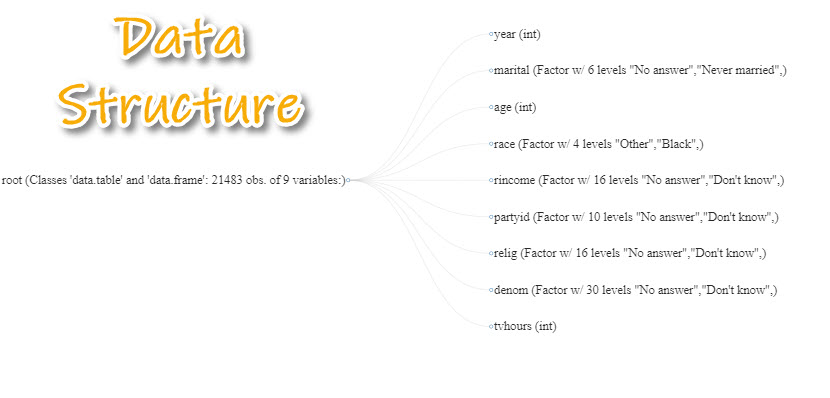
2. Data Structure
Get the code.
Next, we can examine each of the columns specifically learning about what data types are contained inside each of the columns.
- This is really important when we need to know a bit more detail about our data.
- We can begin to hypothesize what we should do to get it into the correct structure for analysis.
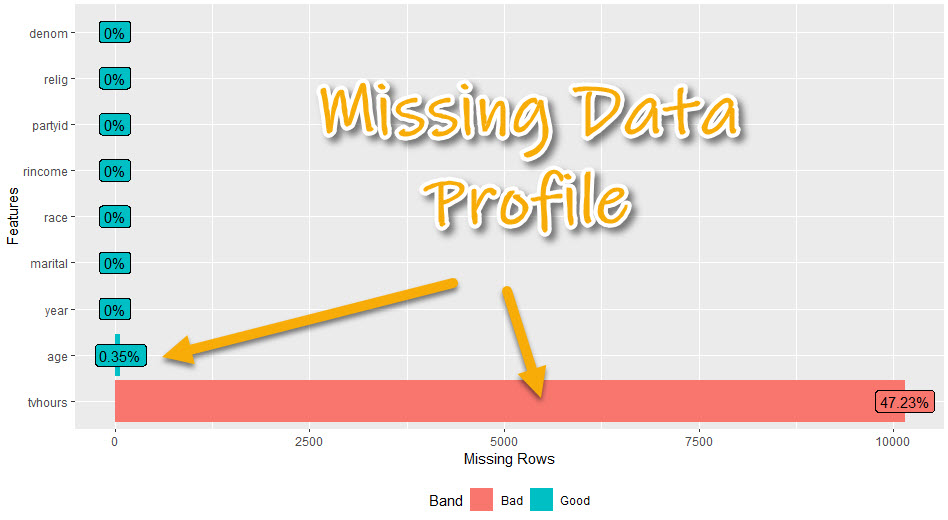
3. Missing Data Profile
Get the code.
The missing data profile report helps us understand which columns have missing data.
- We can start to think about missing data treatment - imputation strategies or if we will need to remove columns
- We can see if columns have hardly any or no missing data - which will be easier to use
- We can see if columns have a lot of missing data - which may need to be removed or heavily treated
4. Univariate Distributions
We have a bunch of options here, which can be used to dive into the columns. I’ll focus on the 2 most important:
- Continuous Features: Histogram
- Categorical Features: Bar Plot
4A. Continuous Features (Histogram)
We can check out the distribution within the numeric data to quickly see what we are dealing with.
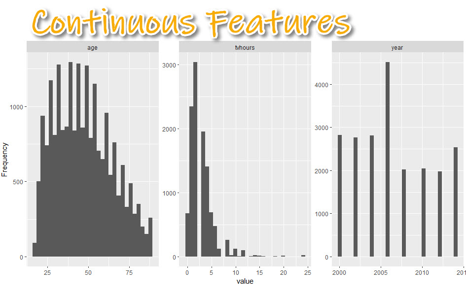
Get the code.
We can get a sense of the distribution of the numeric data.
- Skewed data: TV Hours is very skewed with a few outliers (e.g. watching 24-hours of TV per day)
- Non-normal data: Age tends to be more 25-50 year old respondents than over 50
- Data Range: We can see the survey results go from year 200 to 2014. It looks like every 2-years.
4.B Categorical Features (Bar Plots)
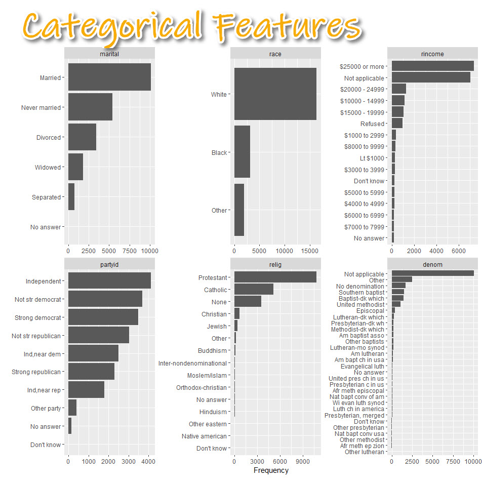
Get the code.
The categorical feature distributions are frequency counts by category shown as a box plot. This helps us:
- Understand categorical distribution: Categories tend to have some levels that are highly present and others that are much more rare.
- Start thinking about categorical treatment: We may need to lump some categories together before modeling.
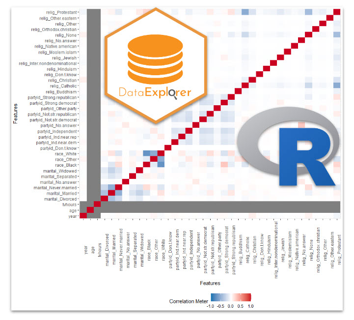
5. Correlation Analysis
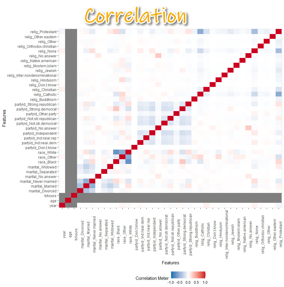
Get the code.
- Correlation helps us tell whether we should move onto modeling.
- Warning! The correlation can be a bit misleading. Many correlations of numeric variables are non-linear. For example, middle-aged people may be more likely to watch less TV. But young and older people may be more likely to watch more TV. The correlation could be low because of the nonlinear relationship.
6. Principal Components
Plotting principal components can help you determine if the data can be compressed. I’ll explain what I mean by this.
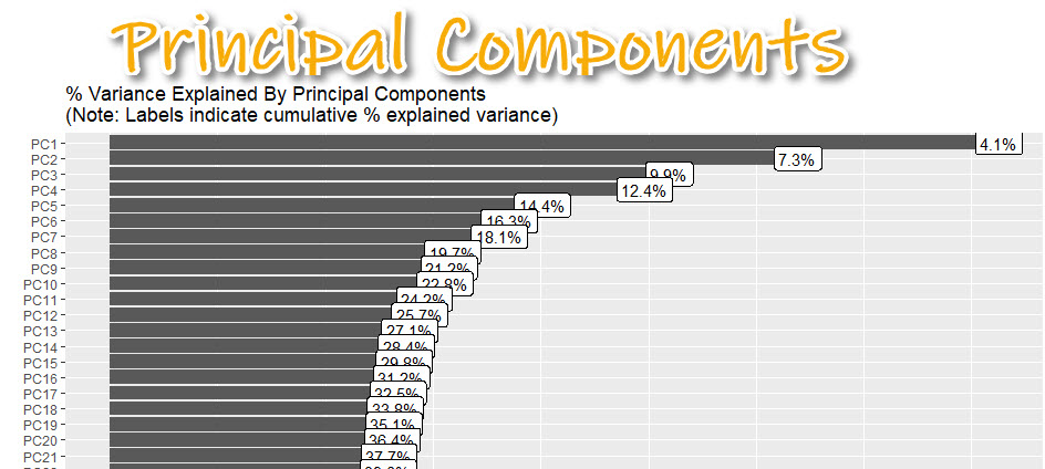
Get the code.
Data that is very wide (many columns) can be computationally expensive to model.
- By applying PCA (Principal Component Analysis), we can determine if compressing using an algorithm like PCA or UMAP is appropriate.
- Here I can see about 37% of the variance explained is contained in the first 20 principal components.
7. Bivariate Distributions
Now we are going to focus on how each feature varies with the target (rincome - how much each person/household makes in annual income).
- Box Plot: For analyzing numeric vs categorical
- Scatter Plot: For analyzing numeric vs numeric (not shown)
Box Plot: Numeric vs Categorical
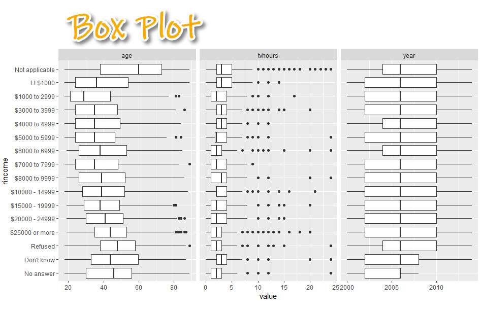
Get the code.
With the box plot, we can:
- Begin to visualize relationships.
- See how each numeric feature (age, tv hours, year) has a relationship with rincome
- $250,000 (high income earners) tend to be in their early 40’s while low income earners are in their late 20’s
Conclusion
You learned how to use the DataExplorer library to automatically create an exploratory data analysis report. Great work! But, there’s a lot more to becoming a data scientist.
If you’d like to become a data scientist (and have an awesome career, improve your quality of life, enjoy your job, and all the fun that comes along), then I can help with that.
Need to advance your business data science skills?
I’ve helped 6,107+ students learn data science for business from an elite business consultant’s perspective.
I’ve worked with Fortune 500 companies like S&P Global, Apple, MRM McCann, and more.
And I built a training program that gets my students life-changing data science careers (don’t believe me? see my testimonials here):
6-Figure Data Science Job at CVS Health ($125K)
Senior VP Of Analytics At JP Morgan ($200K)
50%+ Raises & Promotions ($150K)
Lead Data Scientist at Northwestern Mutual ($175K)
2X-ed Salary (From $60K to $120K)
2 Competing ML Job Offers ($150K)
Promotion to Lead Data Scientist ($175K)
Data Scientist Job at Verizon ($125K+)
Data Scientist Job at CitiBank ($100K + Bonus)
Whenever you are ready, here’s the system they are taking:
Here’s the system that has gotten aspiring data scientists, career transitioners, and life long learners data science jobs and promotions…

Join My 5-Course R-Track Program Now!
(And Become The Data Scientist You Were Meant To Be...)
P.S. - Samantha landed her NEW Data Science R Developer job at CVS Health (Fortune 500). This could be you.