orderSimulatoR: Simulate Orders for Business Analytics
Written
In this post, we will be discussing orderSimulatoR, which enables fast and easy R order simulation for customer and product learning. The basic premise is to simulate data that you’d retrieve from a SQL query of an ERP system. The data can then be merged with products and customers tables to data mine. I’ll go through the basic steps to create an order data set that combines customers and products, and I’ll wrap up with some visualizations to show how you can use order data to expose trends. You can get the scripts and the Cannondale bikes data set at the orderSimulatoR GitHub repository. In case you are wondering what simulated orders look like, click here to scroll to the end result.
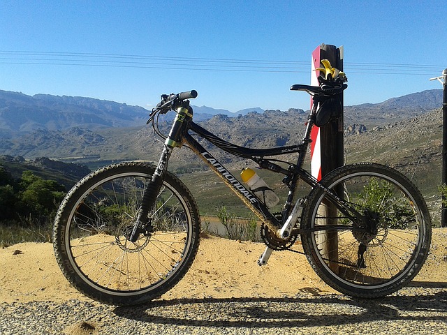
About the Photo:
The bicycle in the photo is one of Cannondale’s top-of-the-line cross-country mountain bikes, the Scalpel. The orderSimulatoR scripts were used to create the Cannondale bikes data set, which simulates orders for the bicycle manufacturer, Cannondale. The data set uses their 2016 models. For more information, visit their website at www.cannondale.com.
Table of Contents
Why orderSimulatoR?
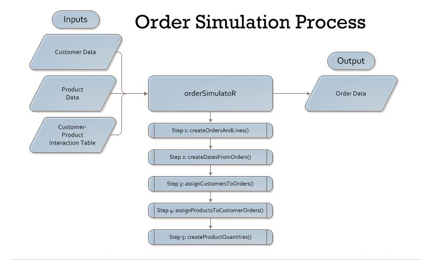
It’s very difficult to create order data with trends for data mining and visualization. I’ve searched for good data sets, and I’ve come to the conclusion that I’m better off creating my own orders data for analyzing on my blog. In the process, I made a collection of R scripts that became known as orderSimulatoR. The scripts are publicly available so others can simulate orders for customers and products in any sales/marketing situation. The process to create orders (shown below) is fast and easy, and the result is orders with customized trends depending on the inputs you create and the parameters you select.
Getting Started
Prior to starting, you’ll need three data frames:
- Customers
- Products
- Customer-Product Interactions
I’ll briefly go through each using the Cannondale bikes data set. If you’re following along, you can access the excel files here. Alternatively, you can generate your own data frames of customers, products and customer-production interactions. Note that the orders.xlsx file is what we will be generating in data frame form. The code below loads the three data frames.
library(xlsx) # For read.xlsx() function

# Read inputs to orderSimulatoR process
customers <- read.xlsx("./data/bikeshops.xlsx", sheetIndex = 1)
products <- read.xlsx("./data/bikes.xlsx", sheetIndex = 1)
customerProductProbs <- read.xlsx("./data/customer_product_interactions.xlsx",
                                  sheetIndex = 1,
                                  startRow = 15)

# Format inputs; Remove unnecessary columns
customerProductProbs <- customerProductProbs[,-(2:11)]
Customers
The customers for the example case are bike shops scattered throughout the United States. I’ve included id, name, city state, latitude, and longitude. The id is important and must be in the first column for the orderSimulatoR scripts to work. The other features are up to you. Feel free to get creative when designing your customers data frame by adding features such as region, size, type, etc that would normally be found in a CRM / ERP system. While features beyond the id are not required for the scripts, it’s a good idea to add them now for data mining later. The first six customer records are shown below.
library(knitr) # used for kable() function

# Show customers dataframe
kable(head(customers))
| bikeshop.id |
bikeshop.name |
bikeshop.city |
bikeshop.state |
latitude |
longitude |
| 1 |
Pittsburgh Mountain Machines |
Pittsburgh |
PA |
40.44062 |
-79.99589 |
| 2 |
Ithaca Mountain Climbers |
Ithaca |
NY |
42.44396 |
-76.50188 |
| 3 |
Columbus Race Equipment |
Columbus |
OH |
39.96118 |
-82.99879 |
| 4 |
Detroit Cycles |
Detroit |
MI |
42.33143 |
-83.04575 |
| 5 |
Cincinnati Speed |
Cincinnati |
OH |
39.10312 |
-84.51202 |
| 6 |
Louisville Race Equipment |
Louisville |
KY |
38.25267 |
-85.75846 |
Products
The products for the example case are road and mountain bikes made by Cannondale, a premier bicycle manufacturer. I’ve included the id and several other features I found on the website including model, category1 (Road, Mountain), category2 (Elite Road, Endurance Road, etc), frame (Carbon, Aluminum), and price. Again, id is the most important feature and must be in the first column for the scripts to work. As with customers, get creative with the features. We’ll use the features when developing the product-customer interactions, which creates the trends that we’ll data mine. The first six products are shown below.
# Show products data frame
kable(head(products))
| bike.id |
model |
category1 |
category2 |
frame |
price |
| 1 |
Supersix Evo Black Inc. |
Road |
Elite Road |
Carbon |
12790 |
| 2 |
Supersix Evo Hi-Mod Team |
Road |
Elite Road |
Carbon |
10660 |
| 3 |
Supersix Evo Hi-Mod Dura Ace 1 |
Road |
Elite Road |
Carbon |
7990 |
| 4 |
Supersix Evo Hi-Mod Dura Ace 2 |
Road |
Elite Road |
Carbon |
5330 |
| 5 |
Supersix Evo Hi-Mod Utegra |
Road |
Elite Road |
Carbon |
4260 |
| 6 |
Supersix Evo Red |
Road |
Elite Road |
Carbon |
3940 |
Customer-Product Interactions
The customer-products interactions is a matrix that links the probability of each customer to purchasing each product (i.e. it is a model for each customer’s purchasing preference). The scripts use this matrix to assign products to orders. The probabilities are critical as these will be what create the customer trends in the data. It’s a good idea to check out the excel spreadsheet, customer_product_interactions.xlsx, which has detailed notes on how to add trends into the customer-product interactions. For the bikes data set, the customers each had a preference for bike style (Road, Mountain, or AnyStyle) and a price range (High and Low). The excel functions assign various probabilities based on how the customer preferences match the product features. A few important points:
- Product id must be the first column
- All subsequent columns should be the customers in order of customer id from 1 to the last customer id.
- Each customer column should sum to 1.0, as this is the product probability density for each customer.
The customer product interactions are shown for the first six customers and products. The way to interpret the matrix is that customer.id.1 has a 0.986% probability of seleting product.id.1 (bike.id = 1).
# Show customer-product interactions data frame
kable(round(customerProductProbs[1:6, 1:6], 4))
| bike.id |
customer.id.1 |
customer.id.2 |
customer.id.3 |
customer.id.4 |
customer.id.5 |
| 1 |
0.0099 |
0.0099 |
0.0196 |
0.0057 |
0.0196 |
| 2 |
0.0099 |
0.0099 |
0.0196 |
0.0057 |
0.0196 |
| 3 |
0.0099 |
0.0099 |
0.0196 |
0.0057 |
0.0196 |
| 4 |
0.0099 |
0.0099 |
0.0196 |
0.0057 |
0.0196 |
| 5 |
0.0099 |
0.0099 |
0.0196 |
0.0057 |
0.0196 |
| 6 |
0.0099 |
0.0099 |
0.0196 |
0.0057 |
0.0196 |
Creating Customer Orders
Once the customer, product and customer-product interaction data frames are finished, you are ready to create orders. The first thing you’ll need is to load the scripts. The scripts can be found here.
# Source orderSimulatoR scripts
source("./scripts/createOrdersAndLines.R")
source("./scripts/createDatesFromOrders.R")
source("./scripts/assignCustomersToOrders.R")
source("./scripts/assignProductsToCustomerOrders.R")
source("./scripts/createProductQuantities.R")
Step 1: Create Orders and Lines
First, we’ll create the orders and lines using the createOrdersAndLines() function. For those unfamiliar with lines, each order typically has several products purchased which are denoted “lines”. The function parameters are number of orders n, max number of lines maxLines, and rate, which affects the distribution of lines on an order.
Quick Digression on the rate Parameter:
This section gets a little technical, so feel free to skip and you won’t miss much.
Several other orderSimulatoR functions use a similar rate parameter, and I recommend playing around with the rates to see how the distribution is affected. The following code generates the probabilities of lines to an order:
# Showing effect of rate on probability of assigning number of lines to orders
maxLines = 10
rate = 1
for (i in 1:maxLines) {
        lineProb[i] <- 1/i^rate
}
lineProb <- lineProb/sum(lineProb)
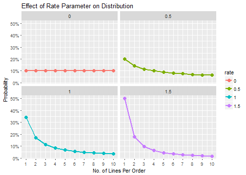
The equation iterates through the number of lines to an order, \(i\), from 1 to maxLines in the equation:
\[lineProb_i = \frac{1}{i^{rate}}\]
Where \(i\) is the number of lines to an order, and \(rate\) is the adjustment parameter. As the number of lines to an order, \(i\), increases, the probability naturally decreases. Because \(i\) is raised to the \(rate\) parameter, the \(rate\) determines how fast or slow the distribution decreases. Larger values cause the distribution to decrease faster, and values close to zero cause the distribution to become more uniform.
The effect of rate adjustment can be conveyed by plotting the probability distribution of orders with maxLines = 10 while adjusting the rate parameter from 0 to 1.5. At rate = 0, the probability of a one-line order is 10%, while at a rate of 1.5 the probability is 50%.
Back to Creating Orders and Lines:
With inputs of n = 2000, maxLines = 30, and rate = 1, the output is a data frame with 2000 orders with 15,644 total rows for each product purchase. Some orders have more lines (more product purchases) and others have less (as dictated by the rate parameter). One note worth mentioning is that the maxLines cannot exceed the number of products (otherwise an order would have more lines than products available which does not make sense).
# Step 1 - Create orders
orders <- createOrdersAndLines(n = 2000, maxLines = 30, rate = 1)
# Data frame for first 3 orders shown
kable(orders[orders$order.id %in% c(1:3),])
| order.id |
order.line |
| 1 |
1 |
| 1 |
2 |
| 2 |
1 |
| 2 |
2 |
| 3 |
1 |
| 3 |
2 |
| 3 |
3 |
| 3 |
4 |
| 3 |
5 |
Step 2: Add Dates to the Orders
Orders typically have a date recorded so the sales can be tracked by time period (e.g. for assessment of time-based metrics like sales by month, quarter, year, etc). As such, we’ll add dates according the distribution of orders in a given year using the createDatesFromOrders() function, which takes four parameters: the orders data frame from Step 1, a startYear, a yearlyOrderDist, and a monthlyOrderDist. The startYear identifies the beginning of the time span, and the length of the yearlyOrderDist (length = 5) creates orders spanning five years. Yearly growth/contraction in sales is simulated using the yearlyOrderDist distribution vector, while seasonality is simulated using the monthlyOrderDist distribution vector. As shown below, we now have dates added according to our desired yearly and monthly distributions.
# Step 2 - Add dates to the orders
orders <- createDatesFromOrders(orders,
                                startYear = 2011,
                                yearlyOrderDist = c(.16, .18, .22, .20, .24),
                                monthlyOrderDist = c(0.045,
                                                     0.075,
                                                     0.100,
                                                     0.110,
                                                     0.120,
                                                     0.125,
                                                     0.100,
                                                     0.085,
                                                     0.075,
                                                     0.060,
                                                     0.060,
                                                     0.045))
# Top of orders data frame showing beginning dates
kable(head(orders))
| order.id |
order.line |
order.date |
| 1 |
1 |
2011-01-07 |
| 1 |
2 |
2011-01-07 |
| 2 |
1 |
2011-01-10 |
| 2 |
2 |
2011-01-10 |
| 3 |
1 |
2011-01-10 |
| 3 |
2 |
2011-01-10 |
The script takes into account no sales on weekends, but does not account for holidays (e.g. Christmas, Thanksgiving, etc). The last six rows of the orders data frame are shown below.
# Bottom of orders data frame showing ending dates
kable(tail(orders))
| |
order.id |
order.line |
order.date |
| 15639 |
2000 |
3 |
2015-12-25 |
| 15640 |
2000 |
4 |
2015-12-25 |
| 15641 |
2000 |
5 |
2015-12-25 |
| 15642 |
2000 |
6 |
2015-12-25 |
| 15643 |
2000 |
7 |
2015-12-25 |
| 15644 |
2000 |
8 |
2015-12-25 |
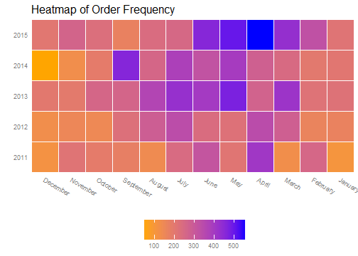
We can use a heatmap to graphically view the order distribution by year and month to get an idea for how the order dates were assigned. As expected, the seasonality of orders follows the monthlyOrderDist distribution, with the majority of orders coming in March through July. The orders increase following the yearlyOrderDist distribution.
Step 3: Assign Customers to Orders
Next, we’ll assign customers to orders using the assignCustomersToOrders() function. The parameters needed are the orders data frame from Step 2, the customers data frame, and the rate parameter, which controls the distribution of orders assigned to customers. Similar to the rate parameter in Step 1, a larger rate increases the number of orders assigned to the largest customers, and as the rate decreases to zero the distribution approaches a uniform distribution. As shown below, orders now have customer id’s.
# Step 3 - Assign customers to the orders
orders <- assignCustomersToOrders(orders, customers, rate = 0.8)
# Data frame for first 3 orders shown
kable(orders[orders$order.id %in% c(1:3),])
| order.id |
order.line |
order.date |
customer.id |
| 1 |
1 |
2011-01-07 |
2 |
| 1 |
2 |
2011-01-07 |
2 |
| 2 |
1 |
2011-01-10 |
10 |
| 2 |
2 |
2011-01-10 |
10 |
| 3 |
1 |
2011-01-10 |
6 |
| 3 |
2 |
2011-01-10 |
6 |
| 3 |
3 |
2011-01-10 |
6 |
| 3 |
4 |
2011-01-10 |
6 |
| 3 |
5 |
2011-01-10 |
6 |
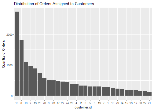
Using a rate = 0.8 still assigns a wide range of orders to customers, and we can see the distribution of order rows by customer in the plot below. Customer 10 has the most order rows at 2731, while Customer 21 has the least order rows at 108.
Step 4: Assign Products to Orders Lines
In step 4, we’ll assign products to the orders using the customer-product interaction table. Keep in mind that this is the critical step where a well-thought-out customer-product interaction table will allow us to uncover deep trends and insights into customer behavior. The assignProductsToCustomerOrders() function takes two arguments: the orders data frame from Step 3 and the customerProductProbs table, which contains the matrix of probabilities linking product.id to customer.id.
# Step 4 - Assign products to orders
orders <- assignProductsToCustomerOrders(orders, customerProductProbs)
# Data frame for first 3 orders shown
kable(orders[orders$order.id %in% c(1:3),])
| order.id |
order.line |
order.date |
customer.id |
product.id |
| 1 |
1 |
2011-01-07 |
2 |
48 |
| 1 |
2 |
2011-01-07 |
2 |
52 |
| 2 |
1 |
2011-01-10 |
10 |
76 |
| 2 |
2 |
2011-01-10 |
10 |
52 |
| 3 |
1 |
2011-01-10 |
6 |
2 |
| 3 |
2 |
2011-01-10 |
6 |
50 |
| 3 |
3 |
2011-01-10 |
6 |
1 |
| 3 |
4 |
2011-01-10 |
6 |
4 |
| 3 |
5 |
2011-01-10 |
6 |
34 |
Step 5: Assign Quantities to Order Lines
In the last step, we assign quantities to the order lines using the createProductQuantities() function. The function takes three parameters: the orders data frame from Step 4, the maxQty, and the rate. The maxQty parameter limits the quantity of products on a order line while the rate parameter controls the distribution. A maxQty = 10 and a rate = 3 places an 83.5% probability on a line quantity of 1, whereas a line quantity of 10 (maximum quantity) has a 0.08% probability.
# Step 5 - Create product quantities
orders <- createProductQuantities(orders, maxQty = 10, rate = 3)
# Data frame for first 3 orders shown
kable(orders[orders$order.id %in% c(1:3),])
| order.id |
order.line |
order.date |
customer.id |
product.id |
quantity |
| 1 |
1 |
2011-01-07 |
2 |
48 |
1 |
| 1 |
2 |
2011-01-07 |
2 |
52 |
1 |
| 2 |
1 |
2011-01-10 |
10 |
76 |
1 |
| 2 |
2 |
2011-01-10 |
10 |
52 |
1 |
| 3 |
1 |
2011-01-10 |
6 |
2 |
1 |
| 3 |
2 |
2011-01-10 |
6 |
50 |
1 |
| 3 |
3 |
2011-01-10 |
6 |
1 |
1 |
| 3 |
4 |
2011-01-10 |
6 |
4 |
1 |
| 3 |
5 |
2011-01-10 |
6 |
34 |
1 |
Joining Orders with Customers and Products
The orders table alone does not give us much information. For instance, we don’t know the names of the customers, the products purchased, or the sales values. Let’s combine some of the tables to make the information more useful.
# Merge customers and products data with the orders to produce and orders.extended data frame
library(dplyr)

orders.extended <- merge(orders, customers, by.x = "customer.id", by.y="bikeshop.id")
orders.extended <- merge(orders.extended, products, by.x = "product.id", by.y = "bike.id")

orders.extended <- orders.extended %>%
        mutate(price.extended = price * quantity) %>%
        select(order.date, order.id, order.line, bikeshop.name, model,
               quantity, price, price.extended, category1, category2, frame) %>%
        arrange(order.id, order.line)
# Data frame for first 3 orders shown
kable(orders.extended[orders.extended$order.id %in% c(1:3),])
| order.date |
order.id |
order.line |
bikeshop.name |
model |
quantity |
price |
price.extended |
category1 |
category2 |
frame |
| 2011-01-07 |
1 |
1 |
Ithaca Mountain Climbers |
Jekyll Carbon 2 |
1 |
6070 |
6070 |
Mountain |
Over Mountain |
Carbon |
| 2011-01-07 |
1 |
2 |
Ithaca Mountain Climbers |
Trigger Carbon 2 |
1 |
5970 |
5970 |
Mountain |
Over Mountain |
Carbon |
| 2011-01-10 |
2 |
1 |
Kansas City 29ers |
Beast of the East 1 |
1 |
2770 |
2770 |
Mountain |
Trail |
Aluminum |
| 2011-01-10 |
2 |
2 |
Kansas City 29ers |
Trigger Carbon 2 |
1 |
5970 |
5970 |
Mountain |
Over Mountain |
Carbon |
| 2011-01-10 |
3 |
1 |
Louisville Race Equipment |
Supersix Evo Hi-Mod Team |
1 |
10660 |
10660 |
Road |
Elite Road |
Carbon |
| 2011-01-10 |
3 |
2 |
Louisville Race Equipment |
Jekyll Carbon 4 |
1 |
3200 |
3200 |
Mountain |
Over Mountain |
Carbon |
| 2011-01-10 |
3 |
3 |
Louisville Race Equipment |
Supersix Evo Black Inc. |
1 |
12790 |
12790 |
Road |
Elite Road |
Carbon |
| 2011-01-10 |
3 |
4 |
Louisville Race Equipment |
Supersix Evo Hi-Mod Dura Ace 2 |
1 |
5330 |
5330 |
Road |
Elite Road |
Carbon |
| 2011-01-10 |
3 |
5 |
Louisville Race Equipment |
Synapse Disc 105 |
1 |
1570 |
1570 |
Road |
Endurance Road |
Aluminum |
Great. Now this finally looks like orders data that could be retrieved from an ERP system. We are ready to start visualizing and data mining. The last part of this post will go into some high level visualizations for data exploration. Future blog posts will dig much deeper.
Exploring the Orders
If you’ve followed along to this point, we have just created the orders from the bikes data set. Now, we can have some fun! Let’s examine the data set.
Sales Over Time
We’ll first take a look at sales over time using the ggplot2 package.
# Plotting sales over time
library(ggplot2)
library(lubridate)

# Create a sales by year data frame
salesByYear <- orders.extended %>%
  group_by(year = year(order.date)) %>%
  summarize(total.sales = sum(price.extended))

# Use ggplot to plot sales by year
ggplot(salesByYear, aes(x=year, y=total.sales)) +
  geom_bar(stat = "identity") +
  geom_smooth(method = "lm", se = FALSE) +
  labs(title="Sales Over Time", x="Year", y="Sales") +
  scale_y_continuous(labels = scales::dollar) +
  geom_text(aes(ymax=total.sales, label=scales::dollar(total.sales)),
                        vjust=1.5,
                        color="white",
                        size=4)
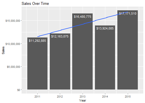
Nice. Cannondale has a general growth trend. It looks like 2015 was Cannondale’s best year with $17,171,510 in total sales!
Top 10 Products
Next, let’s explore some products to get an idea of top sellers.
# Plot top 10 products

# Create top 10 products data frame
productSales <- orders.extended %>%
  group_by(bike.model = model) %>%
  summarize(total.sales = sum(price.extended),
            qty.total = sum(quantity)) %>%
  mutate(pct.total = total.sales / sum(total.sales)) %>%
  arrange(desc(total.sales))
top10.ordered <- head(productSales, 10)
top10.ordered$bike.model <- factor(top10.ordered$bike.model, levels = arrange(top10.ordered, total.sales)$bike.model)

# Use ggplot to plot the top products
ggplot(top10.ordered, aes(x=bike.model, y=total.sales)) +
  geom_bar(stat="identity") +
  geom_text(aes(ymax=pct.total, label=scales::percent(pct.total)),
      hjust= -0.25,
      vjust= 0.5,
      color="black",
      size=4) +
  geom_text(aes(ymax=qty.total, label=paste("Qty:", qty.total)),
      hjust= 1.25,
      vjust= 0.5,
      color="white",
      size=4) +
  coord_flip() +
  labs(title="Top 10 Bike Models",
       x="",
       y="Sales")+
  scale_y_continuous(labels = scales::dollar, limits = c(0,2500000))
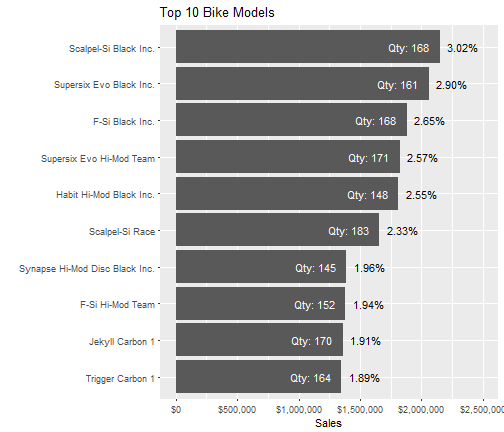
It looks like the best model is the Cannondale Scalpel-Si Black Inc. with 168 units sold representing sales of $2,148,720 or 3.02% of total sales.
Geographic Customer Trends
Finally, we’ll take a look at a map of our customer-base using the leaflet package. The map below charts the customer locations and exposes the sales trends using the circle radius. Larger circles relate to higher sales, and smaller circles relate to lower sales. You can click on the markers to see the bike shop name and sales.
# Plot sales by geographic location

# Create sales by location from orders extedend, joining latitude and longitude
# data by customer name
salesByLocation <- orders.extended %>%
  group_by(bikeshop.name) %>%
  summarise(total.sales = sum(price.extended)) %>%
  left_join(y=customers, by="bikeshop.name") %>%
  mutate(popup = paste0(bikeshop.name, ": ", scales::dollar(total.sales)))

# Use Leaflet package to create map visualizing sales by customer location
library(leaflet)
leaflet(salesByLocation) %>%
  addProviderTiles("CartoDB.Positron") %>%
  addMarkers(lng = ~longitude,
             lat = ~latitude,
             popup = ~popup) %>%
  addCircles(lng = ~longitude,
             lat = ~latitude,
             weight = 2,
             radius = ~(total.sales)^0.775)
This is elightening. Not only is it easy to see who are largest customers are and their locations, but we can see geographic trends. It looks like the southeast US and the midwest are realatively unsaturated geographies. This could be an opportunity to partner with bikeshops in those areas!
Recap
Ok, you’ve made it through a long post, but one that hopefully helps you show off your analytic talents. We discussed how to simulate orders using the orderSimulatoR scripts, which can be used to simulate orders in any situation that has customers and products. All you need is a customer table, products table, and a well-thought-out matrix of probabilities that create the customer-product interaction trends. The simulated orders can then be used for data mining and visualizations. We went through a few high level data visualizations on the bikes data set. We used the ggplot2 and leaflet packages to help understand the overall sales trends, best products, and best customers. With that said, we just scratched the surface of the data mining and visualization process. In future posts, we’ll take a look at more advanced techniques for uncover trends. Until then, onward and upward.
Further Resources
For more R resources, visit R-Bloggers, a site dedicated to R. There’s a wealth of R information, and you may even see this post. Happy analyzing.