Anomaly Detection Using Tidy and Anomalize
Written by Matt Dancho
We recently had an awesome opportunity to work with a great client that asked Business Science to build an open source anomaly detection algorithm that suited their needs. The business goal was to accurately detect anomalies for various marketing data consisting of website actions and marketing feedback spanning thousands of time series across multiple customers and web sources. Enter anomalize: a tidy anomaly detection algorithm that’s time-based (built on top of tibbletime) and scalable from one to many time series!! We are really excited to present this open source R package for others to benefit. In this post, we’ll go through an overview of what anomalize does and how it works.
Case Study: When Open Source Interests Align
We work with many clients teaching data science and using our expertise to accelerate their business. However, it’s rare to have a client’s needs and their willingness to let others benefit align with our interests of pushing the boundaries of data science. This was an exception.
Our client had a challenging problem: detecting anomalies in time series on daily or weekly data at scale. Anomalies indicate exceptional events, which could be increased web traffic in the marketing domain or a malfunctioning server in the IT domain. Regardless, it’s important to flag these unusual occurrences to ensure the business is running smoothly. One of the challenges was that the client deals with not one time series but thousands that need to be analyzed for these extreme events.
An opportunity presented itself to develop an open source package that aligned with our interests of building a scalable adaptation of the Twitter AnomalyDetection package and our client’s desire for a package that would benefit from the open source data science community’s ability to improve over time. The result is anomalize!!!
2 Minutes To Anomalize
We’ve made a short introductory video that’s part of our new Business Science Software Intro Series on YouTube. This will get you up and running in under 2 minutes.
For those of us who prefer to read, here’s the gist of how anomalize works in four simple steps.
Step 1: Install Anomalize
install.packages("anomalize")
Step 2: Load Tidyverse and Anomalize
library(tidyverse)
library(anomalize)
Step 3: Collect Time Series Data
We’ve provided a dataset, tidyverse_cran_downloads, to get you up and running. The dataset consists of daily download counts of 15 “tidyverse” packages.
tidyverse_cran_downloads
## # A tibble: 6,375 x 3
## # Groups:   package [15]
##    date       count package
##    <date>     <dbl> <chr>
##  1 2017-01-01  873. tidyr
##  2 2017-01-02 1840. tidyr
##  3 2017-01-03 2495. tidyr
##  4 2017-01-04 2906. tidyr
##  5 2017-01-05 2847. tidyr
##  6 2017-01-06 2756. tidyr
##  7 2017-01-07 1439. tidyr
##  8 2017-01-08 1556. tidyr
##  9 2017-01-09 3678. tidyr
## 10 2017-01-10 7086. tidyr
## # ... with 6,365 more rows
Step 4: Anomalize
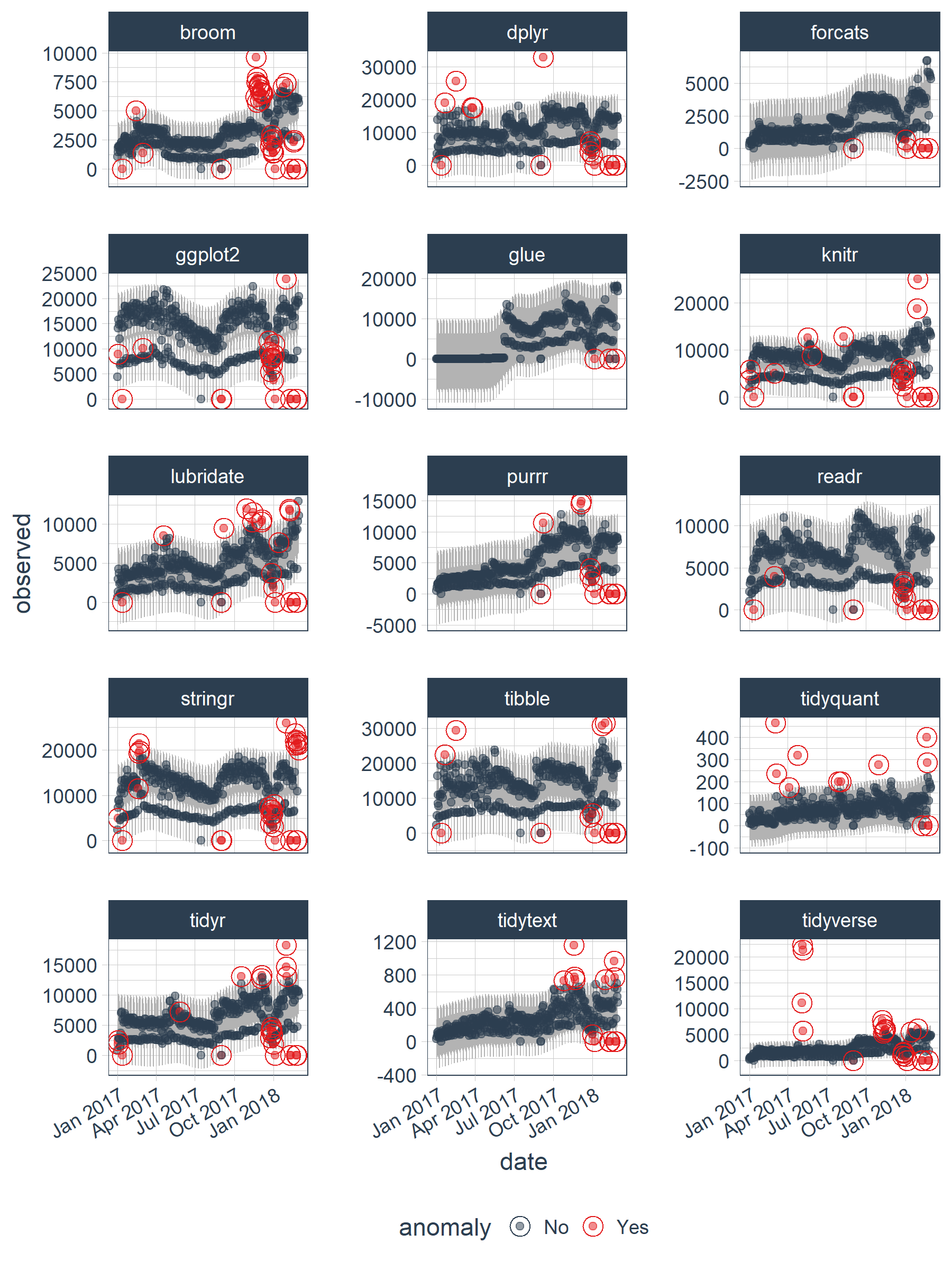
Use the three tidy functions: time_decompose(), anomalize(), and time_recompose() to detect anomalies. Tack on a fourth, plot_anomalies() to visualize.
tidyverse_cran_downloads %>%
    time_decompose(count) %>%
    anomalize(remainder) %>%
    time_recompose() %>%
    plot_anomalies(time_recomposed = TRUE, ncol = 3, alpha_dots = 0.5)
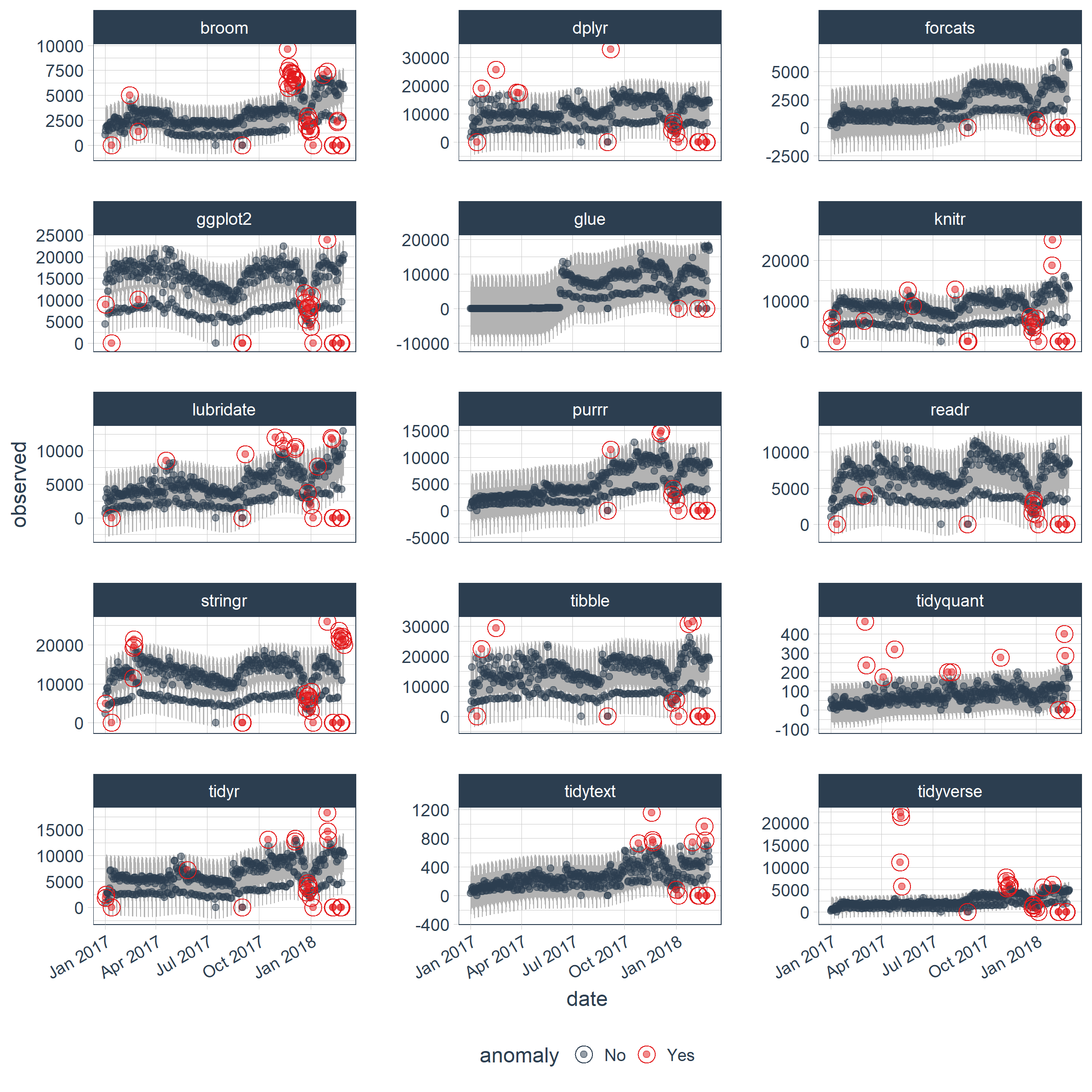
Well that was easy… but, what did we just do???
Anomalize Workflow
You just implemented the “anomalize” (anomaly detection) workflow, which consists of:
- Time series decomposition with
time_decompose()
- Anomaly detection of remainder with
anomalize()
- Anomaly lower and upper bound transformation with
time_recompose()
Time Series Decomposition
The first step is time series decomposition using time_decompose(). The “count” column is decomposed into “observed”, “season”, “trend”, and “remainder” columns. The default values for time series decompose are method = "stl", which is just seasonal decomposition using a Loess smoother (refer to stats::stl()). The frequency and trend parameters are automatically set based on the time scale (or periodicity) of the time series using tibbletime based function under the hood.
tidyverse_cran_downloads %>%
    time_decompose(count, method = "stl", frequency = "auto", trend = "auto")
## # A time tibble: 6,375 x 6
## # Index:  date
## # Groups: package [15]
##    package date       observed season trend remainder
##    <chr>   <date>        <dbl>  <dbl> <dbl>     <dbl>
##  1 tidyr   2017-01-01     873. -2761. 5053.    -1418.
##  2 tidyr   2017-01-02    1840.   901. 5047.    -4108.
##  3 tidyr   2017-01-03    2495.  1460. 5041.    -4006.
##  4 tidyr   2017-01-04    2906.  1430. 5035.    -3559.
##  5 tidyr   2017-01-05    2847.  1239. 5029.    -3421.
##  6 tidyr   2017-01-06    2756.   367. 5024.    -2635.
##  7 tidyr   2017-01-07    1439. -2635. 5018.     -944.
##  8 tidyr   2017-01-08    1556. -2761. 5012.     -695.
##  9 tidyr   2017-01-09    3678.   901. 5006.    -2229.
## 10 tidyr   2017-01-10    7086.  1460. 5000.      626.
## # ... with 6,365 more rows
A nice aspect is that the frequency and trend are automatically selected for you. If you want to see what was selected, set message = TRUE. Also, you can change the selection by inputting a time-based period such as “1 week” or “2 quarters”, which is typically more intuitive that figuring out how many observations fall into a time span. Under the hood, time_frequency() and time_trend() convert these from time-based periods to numeric values using tibbletime!
Anomaly Detection Of Remainder
The next step is to perform anomaly detection on the decomposed data, specifically the “remainder” column. We did this using anomalize(), which produces three new columns: “remainder_l1” (lower limit), “remainder_l2” (upper limit), and “anomaly” (Yes/No Flag). The default method is method = "iqr", which is fast and relatively accurate at detecting anomalies. The alpha parameter is by default set to alpha = 0.05, but can be adjusted to increase or decrease the height of the anomaly bands, making it more difficult or less difficult for data to be anomalous. The max_anoms parameter is by default set to a maximum of max_anoms = 0.2 for 20% of data that can be anomalous. This is the second parameter that can be adjusted. Finally, verbose = FALSE by default which returns a data frame. Try setting verbose = TRUE to get an outlier report as a list.
tidyverse_cran_downloads %>%
    time_decompose(count, method = "stl", frequency = "auto", trend = "auto") %>%
    anomalize(remainder, method = "iqr", alpha = 0.05, max_anoms = 0.2)
## # A time tibble: 6,375 x 9
## # Index:  date
## # Groups: package [15]
##    package date       observed season trend remainder remainder_l1
##    <chr>   <date>        <dbl>  <dbl> <dbl>     <dbl>        <dbl>
##  1 tidyr   2017-01-01     873. -2761. 5053.    -1418.       -3748.
##  2 tidyr   2017-01-02    1840.   901. 5047.    -4108.       -3748.
##  3 tidyr   2017-01-03    2495.  1460. 5041.    -4006.       -3748.
##  4 tidyr   2017-01-04    2906.  1430. 5035.    -3559.       -3748.
##  5 tidyr   2017-01-05    2847.  1239. 5029.    -3421.       -3748.
##  6 tidyr   2017-01-06    2756.   367. 5024.    -2635.       -3748.
##  7 tidyr   2017-01-07    1439. -2635. 5018.     -944.       -3748.
##  8 tidyr   2017-01-08    1556. -2761. 5012.     -695.       -3748.
##  9 tidyr   2017-01-09    3678.   901. 5006.    -2229.       -3748.
## 10 tidyr   2017-01-10    7086.  1460. 5000.      626.       -3748.
## # ... with 6,365 more rows, and 2 more variables: remainder_l2 <dbl>,
## #   anomaly <chr>
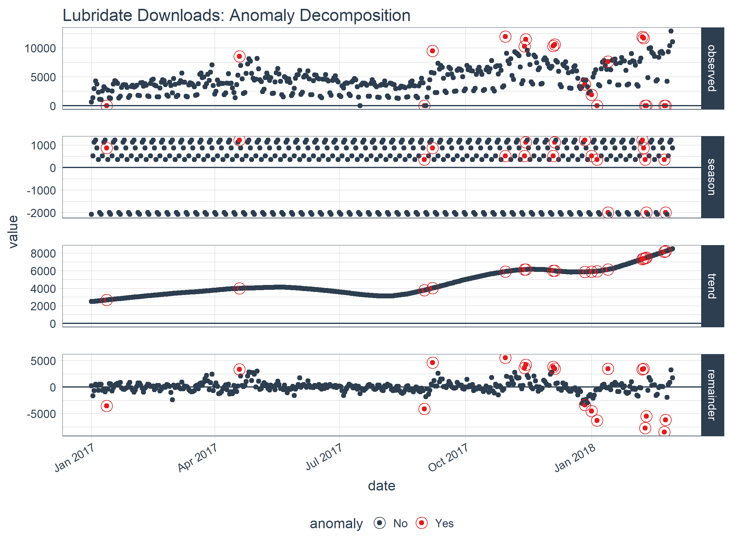
If you want to visualize what’s happening, now’s a good point to try out another plotting function, plot_anomaly_decomposition(). It only works on a single time series so we’ll need to select just one to review. The “season” is removing the weekly cyclic seasonality. The trend is smooth, which is desirable to remove the central tendency without overfitting. Finally, the remainder is analyzed for anomalies detecting the most significant outliers.
tidyverse_cran_downloads %>%

    # Select a single time series
    filter(package == "lubridate") %>%
    ungroup() %>%

    # Anomalize
    time_decompose(count, method = "stl", frequency = "auto", trend = "auto") %>%
    anomalize(remainder, method = "iqr", alpha = 0.05, max_anoms = 0.2) %>%

    # Plot Anomaly Decomposition
    plot_anomaly_decomposition() +
    ggtitle("Lubridate Downloads: Anomaly Decomposition")
Anomaly Lower and Upper Bounds
The last step is to create the lower and upper bounds around the “observed” values. This is the work of time_recompose(), which recomposes the lower and upper bounds of the anomalies around the observed values. Two new columns were created: “recomposed_l1” (lower limit) and “recomposed_l2” (upper limit).
tidyverse_cran_downloads %>%
    time_decompose(count, method = "stl", frequency = "auto", trend = "auto") %>%
    anomalize(remainder, method = "iqr", alpha = 0.05, max_anoms = 0.2) %>%
    time_recompose()
## # A time tibble: 6,375 x 11
## # Index:  date
## # Groups: package [15]
##    package date       observed season trend remainder remainder_l1
##    <chr>   <date>        <dbl>  <dbl> <dbl>     <dbl>        <dbl>
##  1 tidyr   2017-01-01     873. -2761. 5053.    -1418.       -3748.
##  2 tidyr   2017-01-02    1840.   901. 5047.    -4108.       -3748.
##  3 tidyr   2017-01-03    2495.  1460. 5041.    -4006.       -3748.
##  4 tidyr   2017-01-04    2906.  1430. 5035.    -3559.       -3748.
##  5 tidyr   2017-01-05    2847.  1239. 5029.    -3421.       -3748.
##  6 tidyr   2017-01-06    2756.   367. 5024.    -2635.       -3748.
##  7 tidyr   2017-01-07    1439. -2635. 5018.     -944.       -3748.
##  8 tidyr   2017-01-08    1556. -2761. 5012.     -695.       -3748.
##  9 tidyr   2017-01-09    3678.   901. 5006.    -2229.       -3748.
## 10 tidyr   2017-01-10    7086.  1460. 5000.      626.       -3748.
## # ... with 6,365 more rows, and 4 more variables: remainder_l2 <dbl>,
## #   anomaly <chr>, recomposed_l1 <dbl>, recomposed_l2 <dbl>
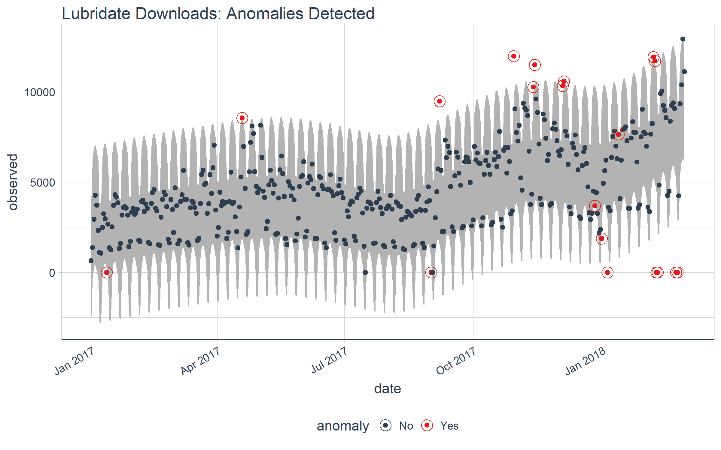
Let’s visualize on just the “lubridate” data. We can do so using plot_anomalies() and setting time_recomposed = TRUE. This function works on both single and grouped data.
tidyverse_cran_downloads %>%
    # Select single time series
    filter(package == "lubridate") %>%
    ungroup() %>%
    # Anomalize
    time_decompose(count, method = "stl", frequency = "auto", trend = "auto") %>%
    anomalize(remainder, method = "iqr", alpha = 0.05, max_anoms = 0.2) %>%
    time_recompose() %>%
    # Plot Anomaly Decomposition
    plot_anomalies(time_recomposed = TRUE) +
    ggtitle("Lubridate Downloads: Anomalies Detected")
That’s it. Once you have the “anomalize workflow” down, you’re ready to detect anomalies!
Packages That Helped In Development
The first thing we did after getting this request was to investigate what methods are currently available. The last thing we wanted to do was solve a problem that’s old news. We were aware of three excellent open source tools:
- Twitter’s
AnomalyDetection package: Available on GitHub.
- Rob Hyndman’s
forecast::tsoutliers() function available on through the forecast package on CRAN.
- Javier Lopez-de-Lacalle’s package,
tsoutliers, on CRAN.
We have worked with all of these R packages and functions before, and each presented learning opportunities that could be integrated into a scalable workflow.
What we liked about Twitter’s AnomalyDetection was that it used two methods in tandem that work extremely well for time series. The “Twitter” method uses time series decomposition (i.e. stats::stl()) but instead of subtracting the Loess trend, it uses the piece-wise median of the data (one or several medians split at specified intervals). The other method that AnomalyDetection employs is the use of Generalized Extreme Studentized Deviate (GESD) as a way of detecting outliers. GESD is nice because it is resistant to the high leverage points that tend to pull a mean or even median in the direction of the most significant outliers. The package works very well with stationary data or even data with trend. However, the package was not built with a tidy interface making it difficult to scale.
Forecast tsoutliers() Function
The tsoutliers() function from the forecast package is a great way to efficiently collect outliers for cleaning prior to performing forecasts. It uses an outlier detection method based on STL with a 3X inner quartile range around remainder from time series decomposition. It’s very fast because there are a maximum of two iterations to determine the outlier bands. However, it’s not setup for a tidy workflow. Nor does it allow adjustment of the 3X. Some time series may need more or less depending on the magnitude of the variance of the remainders in relation to the magnitude of the outliers.
tsoutliers Package
The tsoutliers package works very effectively on a number of traditional forecast time series for detecting anomalies. However, speed was an issue especially when attempting to scale to multiple time series or with minute or second timestamp data.
Anomalize: Incorporating The Best Of All
In reviewing the available packages, we learned from them all incorporating the best of each:
-
Decomposition Methods: We include two time series decomposition methods: "stl" (using traditional seasonal decomposition by Loess) and "twitter" (using seasonal decomposition with median spans).
-
Anomaly Detection Methods: We include two anomaly detection methods: "iqr" (using an approach similar to the 3X IQR of forecast::tsoutliers()) and "gesd" (using the GESD method employed by Twitter’s AnomalyDetection).
In addition, we’ve made some improvements of our own:
-
Anomalize Scales Well: The workflow is tidy and scales with dplyr groups. The functions operate as expected on grouped time series meaning you can just as easily anomalize 500 time series data sets as a single data set.
-
Visuals For Analyzing Anomalies:
-
We include a way to get bands around the “normal” data separating the outliers. People are visual, and bands are really useful in determining how the methods are working or if we need to make adjustments.
-
We include two plotting functions making it easy to see what’s going on during the “anomalize workflow” and providing a way to assess the affect of “adjusting the knobs” that drive time_decompose() and anomalize().
-
Time Based:
-
The entire workflow works with tibbletime data set up with a time-based index. This is good because in our experience almost all time data comes with a date or datetime timestamp that’s really important to characteristics of the data.
-
There’s no need to calculate how many observations fall within a frequency span or trend span. We set up time_decompose() to handle frequency and trend using time-based spans such as “1 week” or “2 quarters” (powered by tibbletime).
Conclusions
We hope that the open source community can benefit from anomalize. Our client is very happy with it, and it’s exciting to see that we can continue to build in new features and functionality that everyone can enjoy.
About Business Science
Business Science specializes in “ROI-driven data science”. We offer training, education, coding expertise, and data science consulting related to business and finance. Our latest creation is Business Science University, which is coming soon! In addition, we deliver about 80% of our effort into the open source data science community in the form of software and our Business Science blog. Visit Business Science on the web or contact us to learn more!