How To Complete A Kaggle Competition In 30 Minutes - Home Credit Default Challenge
Written by Matt Dancho
We were very excited when Home Credit teamed up with Kaggle to host the Home Credit Default Risk Competition. Default risk is a topic that impacts all financial institutions, one that machine learning can help solve. We decided to flip the goal of this challenge: Kaggle competitions are performance driven, where a data scientist has months to fine tune a model to get maximum performance. This is not reality. We turned this goal upside down, focusing on a combination of speed, efficiency, and performance.
In the real world businesses have finite schedules for data science projects. Because of this, we redesigned the competition goal to get very good results quickly. We took a look at the top performance (measured by AUC or area under the curve), which is currently around 0.80. We decided to see how quickly we could develop a competitive model. Follow along and learn how we got a model of 0.70 on a Kaggle submission in about 30 minutes with H2O automated machine learning (AutoML)!
Related Business Machine Learning Articles
Learning Trajectory
In this article, we flip the Kaggle Competition goal upside down focusing on a combination of efficiency and performance. Matt shows you how to get a very good model that gets a 0.70 AUC in about 30 minutes of analysis effort.
We kick the project off with an overview of credit default risk. You’ll begin by understanding what credit default risk is and how machine learning can help identify personal loan applications that are likely to lead to default. We’ll also go over why a Kaggle challenge redesign is more representative of what you’ll need to do in the real world.
Next, we’ll go through the process Matt used to build a competitive model in about 30 minutes. This includes about 10 minutes of strategizing and 20 minutes of actual coding. You’ll see how Matt used the following process to efficiently build a high performance model.
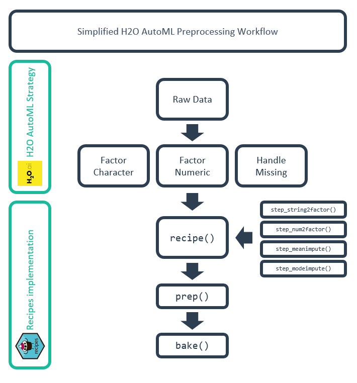
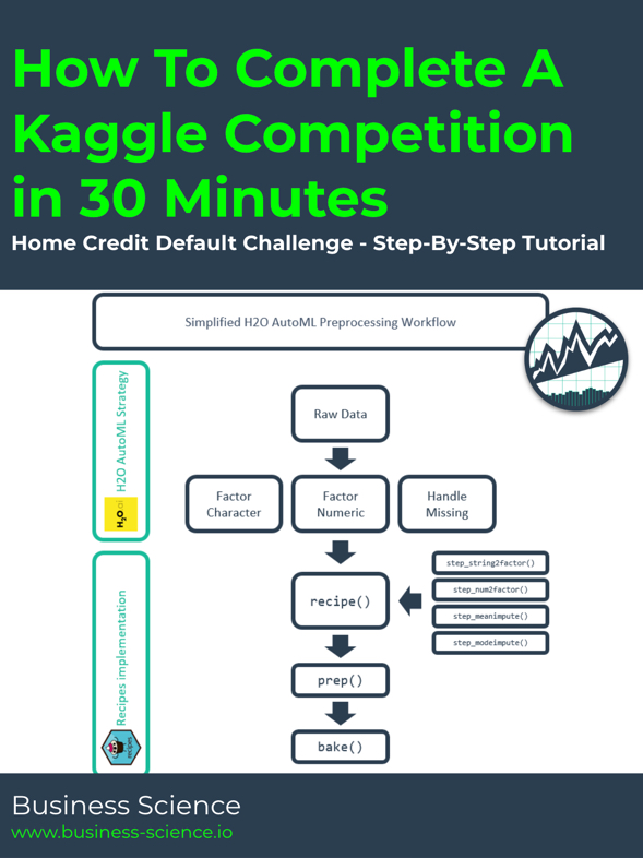
H2O AutoML Preprocessing Workflow
We end on next steps, which provides details on our end-to-end data science project course that will transform your data science abilities in 10 weeks.
Transform Your Abilities In 10 Weeks
If you're interested in learning how to apply critical thinking and data science while solving a real-world business problem following an end-to-end data science project, check out Data Science For Business (DS4B 201-R). Over the course of 10 weeks you will solve an end-to-end Employee Churn data science project following our systematic Business Science Problem Framework.
Get Started Today!
Overview
We’ll briefly touch on what credit default risk is, how machine learning can help, and why a 30-Minute Kaggle Challenge.
What Is Credit Default Risk?
In the world of finance, Credit or Default Risk is the probability that companies or individuals will be unable to make the required payments on their debt obligations. Lenders are exposed to default risk on every extension of credit. Think of financial institutions like Citi, which lend to millions of people worldwide, or JP Morgan Chase & Co, which lend to hundreds of thousands of companies worldwide.

JP Morgan: A Major Lender Of Corporate Loans
Every time Citi or JP Morgan extends a loan to a person or a corporation it assesses the level of risk involved in the transaction. This is because every once in a while people or companies won’t be able to make payments. In the dynamic world we live in unfortunate events happen and circumstances change.
Default risk is comprised of two components:
-
Systemic Risk - The risk related to an external system of interconnected relationships (think of this as the risk associated with they economy, interest rate changes, inflation, recessions, and wars). This risk is often considered unavoidable. The only option is to hedge or not be in the market.
-
Unsystematic Risk - The risk inherent to a person or company (think of this as a company that has a competitor that moves in driving down sales). This risk is avoidable through diversification or making bets on many assets preferably uncorrelated.
In this article, we’ll be focusing on a specific type of risk called Credit or Default Risk, which has both systemic and unsystemic drivers. The main point is that the drivers of default risk can be measured and analyzed for patterns related to default. As a result, the probability of default for a person or an institution is not random. This is where machine learning can help.
The probability of default for a person or an institution is not random. This is where machine learning can help.
Machine Learning For Personal Default Risk
Like any machine learning problem, default risk has drivers, or features related to the person or company that have a relationship with the likelihood of a default. As discussed previously, some of the drivers are systemic and others are unsystemic. Identifying and measuring these drivers are the keys to predicting default.
For the Kaggle Competition, Home Credit (the company) has supplied us with data from several data sources. The following Data Architecture Diagram shows the interrelationships between the data files provided.
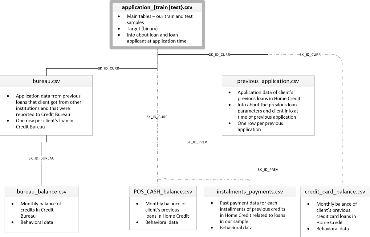
Data Architecture Diagram For Kaggle Home Credit Default Risk Competition
For the purposes of this article, we’ll focus on the application_train.csv and application_test.csv files, which contain a significant amount of useful information for predicting credit default. This is the main source of information for people that have applied for personal loans including features related to their loan application.
Several other data sources are provided such as bureau.csv and previous_application.csv. These data have “one-to-many relationships”, which can be combined through a process called feature engineering. In a tentative future article, we will go into strategies for feature engineering with data that have “one-to-many relationships” (e.g. creating features from bureau.csv that can be combined with application_train.csv).
Why A Kaggle Challenge Redesign?
While we enjoy the idea of the Kaggle Challenge, it’s not representative of a real world scenario where projects have fixed time schedules. The Kaggle Competition goal is to compete on maximum performance. The goal in the real world is quite often to get a good model within a defined project schedule.
Time to completion is important because projects have fixed resources. The longer you are on a project, the more you cost the company money and the more you delay other projects that you could be helping with.
The task of developing a high performance model is just one small piece of a data scientists job. It’s unrealistic to think that an organization will be OK with you (the data scientist) dedicating hundreds of man-hours to squeezing every last drop of performance out of the model. It’s not reality. Refer to the saying, “Great is the enemy of Good”. This is often the case in real-world data science.
Real-World End-To-End Data Science Project Structure
In the real world, you won’t have months that you can dedicate to a model. Rather, you will have maybe a day or two. The majority of your project time will be spent on:
-
Understanding the business (2 weeks)
-
Communicating with decision makers to turn their input into a data collection strategy (2 weeks)
-
Collecting and cleaning the data (1 week to several months)
-
Building a model (1 to 2 days)
-
Converting machine learning results to expected savings or profitability from a business change/improvement and communicating results (1 to 2 weeks)
-
Releasing these results into production via web applications (Several weeks)
This is what we call an “end-to-end” data science project.
Interested in Solving an End-To-End Data Science Project?
If you're interested in learning how to apply critical thinking and data science while solving a real-world business problem following an end-to-end data science project, check out Data Science For Business (DS4B 201-R). Over the course of 10 weeks you will solve an end-to-end Employee Churn data science project following our systematic Business Science Problem Framework.
Get Started Today!
Completing A Kaggle Competition In 30 Minutes
By Matt Dancho, Founder of Business Science
Why 30-minutes for a Kaggle Challenge?
Because I wanted to show you that you that if you leverage high performance tools, you can drastically cut your modeling time down while getting a very good model. As a result, you can spend more time getting better features (up front in the project) and communicating results (after the model is developed). If you get more time after the first round of models are built, you can always go back and improve model performance by adding more data (more features) and improving model performance.
I’ll be providing details how I personally approached the Kaggle Competition and what I did each step of the way to get a good solution fast. Here’s the general process with code that I used to complete a high performing model in about 30 minutes.
Important Note: I did not set out with 30 minutes in mind.
My actual time was roughly 30 minutes.
Basis For Kaggle Competition Redesign
One of my favorite episodes of the Tim Ferris Podcast is one in which he interviews Walter O’Brien, “the real life Scorpion”. Walter is the basis for the hit TV show, Scorpion, that brings together a team of hackers and intellectual misfits to solve crime with technology. While the podcast episode sparked a lot of controversy related to Walter’s history and claims that could not be verified, I found a particular piece of the episode very interesting: The setup of the 1993 Computing Olympics, which Walter reportedly participated in.
In the final challenge of the Computing Olympics, a computer scientist had a fixed amount of time (3 hours) to solve a very complicated business problem by creating an algorithm. The best contestants followed this strategy:
-
The top contestants began by critically thinking: Thinking about the problem and what tools they had in their arsenal to solve it. This could be upwards of 50% to 2/3rd of the allotted competition time.
-
They spent the remaining 50% to 1/3rd speed coding: Hammering out their solution, converting to code with the programming languages that they knew would be the best tool for the scenario.
There’s a lot of value in this approach because of the critical thinking process and the fact that in the real world you will likely only have a fixed amount of days you can work on a model before the business deadline is hit. I wanted to see if this approach could be applied to the Kaggle Home Credit Default Risk Competition.
Setup And Data (5 min)
This part took about 5 minutes excluding the time to download the data and place it into a folder.
You can collect the data from the Kaggle Home Credit Default Risk Competition site. Just a heads up, the datasets in full total 688MB so we need to be mindful of space but more importantly RAM.
Once the data is downloaded, I added it to a folder in my home directory called “00_data”.
Libraries
I loaded the following libraries to tackle the Kaggle Home Credit Default Risk problem. The tidyverse pulls in dplyr, ggplot2, and several other must-haves (e.g. forcats, purrr, etc). The recipes package is loaded for preprocessing. The h2o package is going to do the heavy lifting via automated machine learning (AutoML).
# General
library(tidyverse)
library(skimr)

# Preprocessing
library(recipes)

# Machine Learning
library(h2o)
Data
Next, I read the data with read_csv(), which takes care of much of the column formats for us.
application_train_tbl <- read_csv("00_data/application_train.csv")
application_test_tbl  <- read_csv("00_data/application_test.csv")
Note that the files size is 158MB. This can be a problem when making multiple copies of this data in R, which can quickly cause us to run out of RAM. A strategy I used was to remove previous iterations of the data as I went through processing. You’ll see me use rm() a lot.
Next, I took a quick slice() of the data to see what features are present. I use kable() to format the table for printing here, but this was not done during the 30 minutes of coding.
application_train_tbl %>%
    slice(1:10) %>%
    knitr::kable()
| SK_ID_CURR |
TARGET |
NAME_CONTRACT_TYPE |
CODE_GENDER |
FLAG_OWN_CAR |
FLAG_OWN_REALTY |
CNT_CHILDREN |
AMT_INCOME_TOTAL |
AMT_CREDIT |
AMT_ANNUITY |
AMT_GOODS_PRICE |
NAME_TYPE_SUITE |
NAME_INCOME_TYPE |
NAME_EDUCATION_TYPE |
NAME_FAMILY_STATUS |
NAME_HOUSING_TYPE |
REGION_POPULATION_RELATIVE |
DAYS_BIRTH |
DAYS_EMPLOYED |
DAYS_REGISTRATION |
DAYS_ID_PUBLISH |
OWN_CAR_AGE |
FLAG_MOBIL |
FLAG_EMP_PHONE |
FLAG_WORK_PHONE |
FLAG_CONT_MOBILE |
FLAG_PHONE |
FLAG_EMAIL |
OCCUPATION_TYPE |
CNT_FAM_MEMBERS |
REGION_RATING_CLIENT |
REGION_RATING_CLIENT_W_CITY |
WEEKDAY_APPR_PROCESS_START |
HOUR_APPR_PROCESS_START |
REG_REGION_NOT_LIVE_REGION |
REG_REGION_NOT_WORK_REGION |
LIVE_REGION_NOT_WORK_REGION |
REG_CITY_NOT_LIVE_CITY |
REG_CITY_NOT_WORK_CITY |
LIVE_CITY_NOT_WORK_CITY |
ORGANIZATION_TYPE |
EXT_SOURCE_1 |
EXT_SOURCE_2 |
EXT_SOURCE_3 |
APARTMENTS_AVG |
BASEMENTAREA_AVG |
YEARS_BEGINEXPLUATATION_AVG |
YEARS_BUILD_AVG |
COMMONAREA_AVG |
ELEVATORS_AVG |
ENTRANCES_AVG |
FLOORSMAX_AVG |
FLOORSMIN_AVG |
LANDAREA_AVG |
LIVINGAPARTMENTS_AVG |
LIVINGAREA_AVG |
NONLIVINGAPARTMENTS_AVG |
NONLIVINGAREA_AVG |
APARTMENTS_MODE |
BASEMENTAREA_MODE |
YEARS_BEGINEXPLUATATION_MODE |
YEARS_BUILD_MODE |
COMMONAREA_MODE |
ELEVATORS_MODE |
ENTRANCES_MODE |
FLOORSMAX_MODE |
FLOORSMIN_MODE |
LANDAREA_MODE |
LIVINGAPARTMENTS_MODE |
LIVINGAREA_MODE |
NONLIVINGAPARTMENTS_MODE |
NONLIVINGAREA_MODE |
APARTMENTS_MEDI |
BASEMENTAREA_MEDI |
YEARS_BEGINEXPLUATATION_MEDI |
YEARS_BUILD_MEDI |
COMMONAREA_MEDI |
ELEVATORS_MEDI |
ENTRANCES_MEDI |
FLOORSMAX_MEDI |
FLOORSMIN_MEDI |
LANDAREA_MEDI |
LIVINGAPARTMENTS_MEDI |
LIVINGAREA_MEDI |
NONLIVINGAPARTMENTS_MEDI |
NONLIVINGAREA_MEDI |
FONDKAPREMONT_MODE |
HOUSETYPE_MODE |
TOTALAREA_MODE |
WALLSMATERIAL_MODE |
EMERGENCYSTATE_MODE |
OBS_30_CNT_SOCIAL_CIRCLE |
DEF_30_CNT_SOCIAL_CIRCLE |
OBS_60_CNT_SOCIAL_CIRCLE |
DEF_60_CNT_SOCIAL_CIRCLE |
DAYS_LAST_PHONE_CHANGE |
FLAG_DOCUMENT_2 |
FLAG_DOCUMENT_3 |
FLAG_DOCUMENT_4 |
FLAG_DOCUMENT_5 |
FLAG_DOCUMENT_6 |
FLAG_DOCUMENT_7 |
FLAG_DOCUMENT_8 |
FLAG_DOCUMENT_9 |
FLAG_DOCUMENT_10 |
FLAG_DOCUMENT_11 |
FLAG_DOCUMENT_12 |
FLAG_DOCUMENT_13 |
FLAG_DOCUMENT_14 |
FLAG_DOCUMENT_15 |
FLAG_DOCUMENT_16 |
FLAG_DOCUMENT_17 |
FLAG_DOCUMENT_18 |
FLAG_DOCUMENT_19 |
FLAG_DOCUMENT_20 |
FLAG_DOCUMENT_21 |
AMT_REQ_CREDIT_BUREAU_HOUR |
AMT_REQ_CREDIT_BUREAU_DAY |
AMT_REQ_CREDIT_BUREAU_WEEK |
AMT_REQ_CREDIT_BUREAU_MON |
AMT_REQ_CREDIT_BUREAU_QRT |
AMT_REQ_CREDIT_BUREAU_YEAR |
| 100002 |
1 |
Cash loans |
M |
N |
Y |
0 |
202500 |
406597.5 |
24700.5 |
351000 |
Unaccompanied |
Working |
Secondary / secondary special |
Single / not married |
House / apartment |
0.018801 |
-9461 |
-637 |
-3648 |
-2120 |
NA |
1 |
1 |
0 |
1 |
1 |
0 |
Laborers |
1 |
2 |
2 |
WEDNESDAY |
10 |
0 |
0 |
0 |
0 |
0 |
0 |
Business Entity Type 3 |
0.0830370 |
0.2629486 |
0.1393758 |
0.0247 |
0.0369 |
0.9722 |
0.6192 |
0.0143 |
0.00 |
0.0690 |
0.0833 |
0.1250 |
0.0369 |
0.0202 |
0.0190 |
0.0000 |
0.0000 |
0.0252 |
0.0383 |
0.9722 |
0.6341 |
0.0144 |
0.0000 |
0.0690 |
0.0833 |
0.1250 |
0.0377 |
0.022 |
0.0198 |
0 |
0 |
0.0250 |
0.0369 |
0.9722 |
0.6243 |
0.0144 |
0.00 |
0.0690 |
0.0833 |
0.1250 |
0.0375 |
0.0205 |
0.0193 |
0.0000 |
0.00 |
reg oper account |
block of flats |
0.0149 |
Stone, brick |
No |
2 |
2 |
2 |
2 |
-1134 |
0 |
1 |
0 |
0 |
0 |
0 |
0 |
0 |
0 |
0 |
0 |
0 |
0 |
0 |
0 |
0 |
0 |
0 |
0 |
0 |
0 |
0 |
0 |
0 |
0 |
1 |
| 100003 |
0 |
Cash loans |
F |
N |
N |
0 |
270000 |
1293502.5 |
35698.5 |
1129500 |
Family |
State servant |
Higher education |
Married |
House / apartment |
0.003541 |
-16765 |
-1188 |
-1186 |
-291 |
NA |
1 |
1 |
0 |
1 |
1 |
0 |
Core staff |
2 |
1 |
1 |
MONDAY |
11 |
0 |
0 |
0 |
0 |
0 |
0 |
School |
0.3112673 |
0.6222458 |
NA |
0.0959 |
0.0529 |
0.9851 |
0.7960 |
0.0605 |
0.08 |
0.0345 |
0.2917 |
0.3333 |
0.0130 |
0.0773 |
0.0549 |
0.0039 |
0.0098 |
0.0924 |
0.0538 |
0.9851 |
0.8040 |
0.0497 |
0.0806 |
0.0345 |
0.2917 |
0.3333 |
0.0128 |
0.079 |
0.0554 |
0 |
0 |
0.0968 |
0.0529 |
0.9851 |
0.7987 |
0.0608 |
0.08 |
0.0345 |
0.2917 |
0.3333 |
0.0132 |
0.0787 |
0.0558 |
0.0039 |
0.01 |
reg oper account |
block of flats |
0.0714 |
Block |
No |
1 |
0 |
1 |
0 |
-828 |
0 |
1 |
0 |
0 |
0 |
0 |
0 |
0 |
0 |
0 |
0 |
0 |
0 |
0 |
0 |
0 |
0 |
0 |
0 |
0 |
0 |
0 |
0 |
0 |
0 |
0 |
| 100004 |
0 |
Revolving loans |
M |
Y |
Y |
0 |
67500 |
135000.0 |
6750.0 |
135000 |
Unaccompanied |
Working |
Secondary / secondary special |
Single / not married |
House / apartment |
0.010032 |
-19046 |
-225 |
-4260 |
-2531 |
26 |
1 |
1 |
1 |
1 |
1 |
0 |
Laborers |
1 |
2 |
2 |
MONDAY |
9 |
0 |
0 |
0 |
0 |
0 |
0 |
Government |
NA |
0.5559121 |
0.7295667 |
NA |
NA |
NA |
NA |
NA |
NA |
NA |
NA |
NA |
NA |
NA |
NA |
NA |
NA |
NA |
NA |
NA |
NA |
NA |
NA |
NA |
NA |
NA |
NA |
NA |
NA |
NA |
NA |
NA |
NA |
NA |
NA |
NA |
NA |
NA |
NA |
NA |
NA |
NA |
NA |
NA |
NA |
NA |
NA |
NA |
NA |
NA |
0 |
0 |
0 |
0 |
-815 |
0 |
0 |
0 |
0 |
0 |
0 |
0 |
0 |
0 |
0 |
0 |
0 |
0 |
0 |
0 |
0 |
0 |
0 |
0 |
0 |
0 |
0 |
0 |
0 |
0 |
0 |
| 100006 |
0 |
Cash loans |
F |
N |
Y |
0 |
135000 |
312682.5 |
29686.5 |
297000 |
Unaccompanied |
Working |
Secondary / secondary special |
Civil marriage |
House / apartment |
0.008019 |
-19005 |
-3039 |
-9833 |
-2437 |
NA |
1 |
1 |
0 |
1 |
0 |
0 |
Laborers |
2 |
2 |
2 |
WEDNESDAY |
17 |
0 |
0 |
0 |
0 |
0 |
0 |
Business Entity Type 3 |
NA |
0.6504417 |
NA |
NA |
NA |
NA |
NA |
NA |
NA |
NA |
NA |
NA |
NA |
NA |
NA |
NA |
NA |
NA |
NA |
NA |
NA |
NA |
NA |
NA |
NA |
NA |
NA |
NA |
NA |
NA |
NA |
NA |
NA |
NA |
NA |
NA |
NA |
NA |
NA |
NA |
NA |
NA |
NA |
NA |
NA |
NA |
NA |
NA |
NA |
NA |
2 |
0 |
2 |
0 |
-617 |
0 |
1 |
0 |
0 |
0 |
0 |
0 |
0 |
0 |
0 |
0 |
0 |
0 |
0 |
0 |
0 |
0 |
0 |
0 |
0 |
NA |
NA |
NA |
NA |
NA |
NA |
| 100007 |
0 |
Cash loans |
M |
N |
Y |
0 |
121500 |
513000.0 |
21865.5 |
513000 |
Unaccompanied |
Working |
Secondary / secondary special |
Single / not married |
House / apartment |
0.028663 |
-19932 |
-3038 |
-4311 |
-3458 |
NA |
1 |
1 |
0 |
1 |
0 |
0 |
Core staff |
1 |
2 |
2 |
THURSDAY |
11 |
0 |
0 |
0 |
0 |
1 |
1 |
Religion |
NA |
0.3227383 |
NA |
NA |
NA |
NA |
NA |
NA |
NA |
NA |
NA |
NA |
NA |
NA |
NA |
NA |
NA |
NA |
NA |
NA |
NA |
NA |
NA |
NA |
NA |
NA |
NA |
NA |
NA |
NA |
NA |
NA |
NA |
NA |
NA |
NA |
NA |
NA |
NA |
NA |
NA |
NA |
NA |
NA |
NA |
NA |
NA |
NA |
NA |
NA |
0 |
0 |
0 |
0 |
-1106 |
0 |
0 |
0 |
0 |
0 |
0 |
1 |
0 |
0 |
0 |
0 |
0 |
0 |
0 |
0 |
0 |
0 |
0 |
0 |
0 |
0 |
0 |
0 |
0 |
0 |
0 |
| 100008 |
0 |
Cash loans |
M |
N |
Y |
0 |
99000 |
490495.5 |
27517.5 |
454500 |
Spouse, partner |
State servant |
Secondary / secondary special |
Married |
House / apartment |
0.035792 |
-16941 |
-1588 |
-4970 |
-477 |
NA |
1 |
1 |
1 |
1 |
1 |
0 |
Laborers |
2 |
2 |
2 |
WEDNESDAY |
16 |
0 |
0 |
0 |
0 |
0 |
0 |
Other |
NA |
0.3542247 |
0.6212263 |
NA |
NA |
NA |
NA |
NA |
NA |
NA |
NA |
NA |
NA |
NA |
NA |
NA |
NA |
NA |
NA |
NA |
NA |
NA |
NA |
NA |
NA |
NA |
NA |
NA |
NA |
NA |
NA |
NA |
NA |
NA |
NA |
NA |
NA |
NA |
NA |
NA |
NA |
NA |
NA |
NA |
NA |
NA |
NA |
NA |
NA |
NA |
0 |
0 |
0 |
0 |
-2536 |
0 |
1 |
0 |
0 |
0 |
0 |
0 |
0 |
0 |
0 |
0 |
0 |
0 |
0 |
0 |
0 |
0 |
0 |
0 |
0 |
0 |
0 |
0 |
0 |
1 |
1 |
| 100009 |
0 |
Cash loans |
F |
Y |
Y |
1 |
171000 |
1560726.0 |
41301.0 |
1395000 |
Unaccompanied |
Commercial associate |
Higher education |
Married |
House / apartment |
0.035792 |
-13778 |
-3130 |
-1213 |
-619 |
17 |
1 |
1 |
0 |
1 |
1 |
0 |
Accountants |
3 |
2 |
2 |
SUNDAY |
16 |
0 |
0 |
0 |
0 |
0 |
0 |
Business Entity Type 3 |
0.7747614 |
0.7239999 |
0.4920601 |
NA |
NA |
NA |
NA |
NA |
NA |
NA |
NA |
NA |
NA |
NA |
NA |
NA |
NA |
NA |
NA |
NA |
NA |
NA |
NA |
NA |
NA |
NA |
NA |
NA |
NA |
NA |
NA |
NA |
NA |
NA |
NA |
NA |
NA |
NA |
NA |
NA |
NA |
NA |
NA |
NA |
NA |
NA |
NA |
NA |
NA |
NA |
1 |
0 |
1 |
0 |
-1562 |
0 |
0 |
0 |
0 |
0 |
0 |
1 |
0 |
0 |
0 |
0 |
0 |
1 |
0 |
0 |
0 |
0 |
0 |
0 |
0 |
0 |
0 |
0 |
1 |
1 |
2 |
| 100010 |
0 |
Cash loans |
M |
Y |
Y |
0 |
360000 |
1530000.0 |
42075.0 |
1530000 |
Unaccompanied |
State servant |
Higher education |
Married |
House / apartment |
0.003122 |
-18850 |
-449 |
-4597 |
-2379 |
8 |
1 |
1 |
1 |
1 |
0 |
0 |
Managers |
2 |
3 |
3 |
MONDAY |
16 |
0 |
0 |
0 |
0 |
1 |
1 |
Other |
NA |
0.7142793 |
0.5406545 |
NA |
NA |
NA |
NA |
NA |
NA |
NA |
NA |
NA |
NA |
NA |
NA |
NA |
NA |
NA |
NA |
NA |
NA |
NA |
NA |
NA |
NA |
NA |
NA |
NA |
NA |
NA |
NA |
NA |
NA |
NA |
NA |
NA |
NA |
NA |
NA |
NA |
NA |
NA |
NA |
NA |
NA |
NA |
NA |
NA |
NA |
NA |
2 |
0 |
2 |
0 |
-1070 |
0 |
1 |
0 |
0 |
0 |
0 |
0 |
0 |
0 |
0 |
0 |
0 |
0 |
0 |
0 |
0 |
0 |
0 |
0 |
0 |
0 |
0 |
0 |
0 |
0 |
0 |
| 100011 |
0 |
Cash loans |
F |
N |
Y |
0 |
112500 |
1019610.0 |
33826.5 |
913500 |
Children |
Pensioner |
Secondary / secondary special |
Married |
House / apartment |
0.018634 |
-20099 |
365243 |
-7427 |
-3514 |
NA |
1 |
0 |
0 |
1 |
0 |
0 |
NA |
2 |
2 |
2 |
WEDNESDAY |
14 |
0 |
0 |
0 |
0 |
0 |
0 |
XNA |
0.5873340 |
0.2057473 |
0.7517237 |
NA |
NA |
NA |
NA |
NA |
NA |
NA |
NA |
NA |
NA |
NA |
NA |
NA |
NA |
NA |
NA |
NA |
NA |
NA |
NA |
NA |
NA |
NA |
NA |
NA |
NA |
NA |
NA |
NA |
NA |
NA |
NA |
NA |
NA |
NA |
NA |
NA |
NA |
NA |
NA |
NA |
NA |
NA |
NA |
NA |
NA |
NA |
1 |
0 |
1 |
0 |
0 |
0 |
1 |
0 |
0 |
0 |
0 |
0 |
0 |
0 |
0 |
0 |
0 |
0 |
0 |
0 |
0 |
0 |
0 |
0 |
0 |
0 |
0 |
0 |
0 |
0 |
1 |
| 100012 |
0 |
Revolving loans |
M |
N |
Y |
0 |
135000 |
405000.0 |
20250.0 |
405000 |
Unaccompanied |
Working |
Secondary / secondary special |
Single / not married |
House / apartment |
0.019689 |
-14469 |
-2019 |
-14437 |
-3992 |
NA |
1 |
1 |
0 |
1 |
0 |
0 |
Laborers |
1 |
2 |
2 |
THURSDAY |
8 |
0 |
0 |
0 |
0 |
0 |
0 |
Electricity |
NA |
0.7466436 |
NA |
NA |
NA |
NA |
NA |
NA |
NA |
NA |
NA |
NA |
NA |
NA |
NA |
NA |
NA |
NA |
NA |
NA |
NA |
NA |
NA |
NA |
NA |
NA |
NA |
NA |
NA |
NA |
NA |
NA |
NA |
NA |
NA |
NA |
NA |
NA |
NA |
NA |
NA |
NA |
NA |
NA |
NA |
NA |
NA |
NA |
NA |
NA |
2 |
0 |
2 |
0 |
-1673 |
0 |
0 |
0 |
0 |
0 |
0 |
0 |
0 |
0 |
0 |
0 |
0 |
0 |
0 |
0 |
0 |
0 |
0 |
0 |
0 |
NA |
NA |
NA |
NA |
NA |
NA |
application_train_tbl: First 10 Rows
A few points about the data:
-
The training data contains 307K observations, which are people applied for and received loans
-
The “TARGET” column identifies whether or not the person defaulted
-
The remaining 121 features describe various attributes about the person, loan, and application
-
There are several additional data sets (bureau.csv, previous_application.csv). I ignored these since most of the important data was likely to be in the main file. These auxiliary files contain data that is one-to-many relationship, which would require aggregation (a feature engineering method) and considerably more work for the unknown benefit.
I was more interested in agile iteration: Building a good model quickly, then going back to try to improve later.
Train And Test Sets
Next, I formatted the data as train and test sets. I noted that the “application_test_tbl” did not have a TARGET column (I found this out when I tried to process it with recipes during the first go-around). The “test” set is the set that the Kaggle Competition is measured against that we will submit later. Note that I remove the unnecessary data sets after I’m finished with them in order to save memory.
# Training data: Separate into x and y tibbles
x_train_tbl <- application_train_tbl %>% select(-TARGET)
y_train_tbl <- application_train_tbl %>% select(TARGET)

# Testing data: What we submit in the competition
x_test_tbl  <- application_test_tbl

# Remove the original data to save memory
rm(application_train_tbl)
rm(application_test_tbl)
Data Inspection
I used one of my favorite packages for data investigation, skimr. This package helps me understand how much missing data I’m dealing with and overall sense of the data by data type.
Normally I just run skim() on the data. However, for the purposes of outputting in a readable format on the web, I’ll use skim_to_list()
skim_to_list(x_train_tbl)
## $integer
## # A tibble: 40 x 12
##    variable  missing complete n      mean   sd     p0    p25   median
##  * <chr>     <chr>   <chr>    <chr>  <chr>  <chr>  <chr> <chr> <chr>
##  1 CNT_CHIL~ 0       307511   307511 "    ~ "    ~ 0     "   ~ 0
##  2 DAYS_BIR~ 0       307511   307511 "-160~ "  43~ -252~ "-19~ -15750
##  3 DAYS_EMP~ 0       307511   307511 " 638~ "1412~ -179~ " -2~ -1213
##  4 DAYS_ID_~ 0       307511   307511 " -29~ "  15~ -7197 " -4~ -3254
##  5 FLAG_CON~ 0       307511   307511 "    ~ "    ~ 0     "   ~ 1
##  6 FLAG_DOC~ 0       307511   307511 "    ~ "    ~ 0     "   ~ 0
##  7 FLAG_DOC~ 0       307511   307511 "    ~ "    ~ 0     "   ~ 0
##  8 FLAG_DOC~ 0       307511   307511 "    ~ "    ~ 0     "   ~ 0
##  9 FLAG_DOC~ 0       307511   307511 "    ~ "    ~ 0     "   ~ 0
## 10 FLAG_DOC~ 0       307511   307511 "    ~ "    ~ 0     "   ~ 0
## # ... with 30 more rows, and 3 more variables: p75 <chr>, p100 <chr>,
## #   hist <chr>
##
## $character
## # A tibble: 16 x 8
##    variable         missing complete n     min   max   empty n_unique
##  * <chr>            <chr>   <chr>    <chr> <chr> <chr> <chr> <chr>
##  1 CODE_GENDER      0       307511   3075~ 1     3     0     3
##  2 EMERGENCYSTATE_~ 145755  161756   3075~ 2     3     0     2
##  3 FLAG_OWN_CAR     0       307511   3075~ 1     1     0     2
##  4 FLAG_OWN_REALTY  0       307511   3075~ 1     1     0     2
##  5 FONDKAPREMONT_M~ 210295  97216    3075~ 13    21    0     4
##  6 HOUSETYPE_MODE   154297  153214   3075~ 14    16    0     3
##  7 NAME_CONTRACT_T~ 0       307511   3075~ 10    15    0     2
##  8 NAME_EDUCATION_~ 0       307511   3075~ 15    29    0     5
##  9 NAME_FAMILY_STA~ 0       307511   3075~ 5     20    0     6
## 10 NAME_HOUSING_TY~ 0       307511   3075~ 12    19    0     6
## 11 NAME_INCOME_TYPE 0       307511   3075~ 7     20    0     8
## 12 NAME_TYPE_SUITE  1292    306219   3075~ 6     15    0     7
## 13 OCCUPATION_TYPE  96391   211120   3075~ 7     21    0     18
## 14 ORGANIZATION_TY~ 0       307511   3075~ 3     22    0     58
## 15 WALLSMATERIAL_M~ 156341  151170   3075~ 5     12    0     7
## 16 WEEKDAY_APPR_PR~ 0       307511   3075~ 6     9     0     7
##
## $numeric
## # A tibble: 65 x 12
##    variable   missing complete n      mean   sd    p0    p25   median
##  * <chr>      <chr>   <chr>    <chr>  <chr>  <chr> <chr> <chr> <chr>
##  1 AMT_ANNUI~ 12      307499   307511 " 271~ " 14~ "  1~ " 16~ " 249~
##  2 AMT_CREDIT 0       307511   307511 " 6e+~ " 4e~ " 45~ "270~ "5135~
##  3 AMT_GOODS~ 278     307233   307511 "5383~ "369~ " 40~ "238~ "4500~
##  4 AMT_INCOM~ 0       307511   307511 "1687~ "237~ " 25~ "112~ "1471~
##  5 AMT_REQ_C~ 41519   265992   307511 "    ~ "   ~ "   ~ "   ~ "    ~
##  6 AMT_REQ_C~ 41519   265992   307511 "    ~ "   ~ "   ~ "   ~ "    ~
##  7 AMT_REQ_C~ 41519   265992   307511 "    ~ "   ~ "   ~ "   ~ "    ~
##  8 AMT_REQ_C~ 41519   265992   307511 "    ~ "   ~ "   ~ "   ~ "    ~
##  9 AMT_REQ_C~ 41519   265992   307511 "    ~ "   ~ "   ~ "   ~ "    ~
## 10 AMT_REQ_C~ 41519   265992   307511 "    ~ "   ~ "   ~ "   ~ "    ~
## # ... with 55 more rows, and 3 more variables: p75 <chr>, p100 <chr>,
## #   hist <chr>
I see that there are 3 data type formats: integer, numeric, and character. For H2O we need numeric and factor. I see some of the integer values are “FLAG”, which typically indicates a factor.
Analysis Strategy (5 min)
The first 5 minutes were dedicated to mocking up a plan for the competition. I began by framing a solution on a piece of scrap paper.
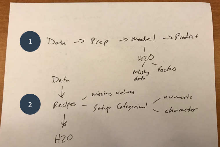
Analysis Strategy on Scrap Paper
The general workflow (1) is at the top where I wanted to accomplish the following goals:
-
Read the data
-
Prepare the data
-
Model - This step I wanted to use H2O because I knew I could leverage automated machine learning (AutoML) to vastly speed up the modeling process.
-
Make predictions
The second half (2) of the scrap paper is how I planned to execute each step. The workflow involved a special tool using recipes to accomplish the preprocessing. I planned to minimally transform the data addressing missing values and categorical data.
With a plan in hand, I got started.
Preprocessing Strategy (5 min)
I leveraged my knowledge of how H2O AutoML works under the hood to develop a simplified strategy to tackle preprocessing. H2O AutoML handles common tasks internally such as creating dummy variables (or one hot encoding), performing statistical transformations (e.g. YeoJohnson), etc. As a result, this greatly simplifies the preprocessing tasks that I needed to worry about.
The main things I focused on were:
-
Character data that needs to be factored: h2o.automl() requires any character data to be converted to a factor.
-
Numeric data that has a low number of unique counts: This is common in business data where there are numeric features that have low number of unique values. These are typically categorical data.
-
Missing values: Missing values need to be either imputed or to have the columns and or rows dropped. I made a point to impute all data before modeling with h2o.automl() although I believe that AutoML has methods for handling missing data.
Here’s the simplified strategy I used for preprocessing for AutoML. I diagrammed it after the fact to show the flow of how the entire process works beyond my “chicken scratch” scrap paper diagram shown previously. Keep in mind that H2O handles most data transformations “under the hood”, which is really useful for getting good models quickly.
H2O AutoML Preprocessing Workflow
Interested in Learning Preprocessing Strategies For Business?
If you're interested in learning how to apply the preprocessing strategies using R Programming beyond the simplified strategy shown, we teach preprocessing with recipes in Chapter 3 of Data Science For Business (DS4B 201-R) as part of our 10-Week end-to-end Employee Churn data science project.
Get Started Today!
Let’s implement the H2O AutoML Preprocessing Workflow shown in the diagram.
Character Data
First, I collected the names of all character data. These columns will be converted into factors.
string_2_factor_names <- x_train_tbl %>%
    select_if(is.character) %>%
    names()

string_2_factor_names
##  [1] "NAME_CONTRACT_TYPE"         "CODE_GENDER"
##  [3] "FLAG_OWN_CAR"               "FLAG_OWN_REALTY"
##  [5] "NAME_TYPE_SUITE"            "NAME_INCOME_TYPE"
##  [7] "NAME_EDUCATION_TYPE"        "NAME_FAMILY_STATUS"
##  [9] "NAME_HOUSING_TYPE"          "OCCUPATION_TYPE"
## [11] "WEEKDAY_APPR_PROCESS_START" "ORGANIZATION_TYPE"
## [13] "FONDKAPREMONT_MODE"         "HOUSETYPE_MODE"
## [15] "WALLSMATERIAL_MODE"         "EMERGENCYSTATE_MODE"
Numeric Factor Data
Next, I looked at which numeric data should be factored (categorical). These typically have a low number of unique levels. I used a few dplyr and purrr operations to get a count of the unique levels. The real trick is using map_df() with the anonymous function ~ unique(.) %>% length(), which counts the unique values in each column, then gather()-ing the results in the long format.
unique_numeric_values_tbl <- x_train_tbl %>%
    select_if(is.numeric) %>%
    map_df(~ unique(.) %>% length()) %>%
    gather() %>%
    arrange(value) %>%
    mutate(key = as_factor(key))

unique_numeric_values_tbl
## # A tibble: 105 x 2
##    key                         value
##    <fct>                       <int>
##  1 FLAG_MOBIL                      2
##  2 FLAG_EMP_PHONE                  2
##  3 FLAG_WORK_PHONE                 2
##  4 FLAG_CONT_MOBILE                2
##  5 FLAG_PHONE                      2
##  6 FLAG_EMAIL                      2
##  7 REG_REGION_NOT_LIVE_REGION      2
##  8 REG_REGION_NOT_WORK_REGION      2
##  9 LIVE_REGION_NOT_WORK_REGION     2
## 10 REG_CITY_NOT_LIVE_CITY          2
## # ... with 95 more rows
I used a factor limit of 7 meaning any values with less than 7 unique observations will not be converted to factors. I then collected the column names by pull()-ing the key column and storing as character data.
factor_limit <- 7

num_2_factor_names <- unique_numeric_values_tbl %>%
    filter(value < factor_limit) %>%
    arrange(desc(value)) %>%
    pull(key) %>%
    as.character()

num_2_factor_names
##  [1] "AMT_REQ_CREDIT_BUREAU_HOUR"  "REGION_RATING_CLIENT"
##  [3] "REGION_RATING_CLIENT_W_CITY" "FLAG_MOBIL"
##  [5] "FLAG_EMP_PHONE"              "FLAG_WORK_PHONE"
##  [7] "FLAG_CONT_MOBILE"            "FLAG_PHONE"
##  [9] "FLAG_EMAIL"                  "REG_REGION_NOT_LIVE_REGION"
## [11] "REG_REGION_NOT_WORK_REGION"  "LIVE_REGION_NOT_WORK_REGION"
## [13] "REG_CITY_NOT_LIVE_CITY"      "REG_CITY_NOT_WORK_CITY"
## [15] "LIVE_CITY_NOT_WORK_CITY"     "FLAG_DOCUMENT_2"
## [17] "FLAG_DOCUMENT_3"             "FLAG_DOCUMENT_4"
## [19] "FLAG_DOCUMENT_5"             "FLAG_DOCUMENT_6"
## [21] "FLAG_DOCUMENT_7"             "FLAG_DOCUMENT_8"
## [23] "FLAG_DOCUMENT_9"             "FLAG_DOCUMENT_10"
## [25] "FLAG_DOCUMENT_11"            "FLAG_DOCUMENT_12"
## [27] "FLAG_DOCUMENT_13"            "FLAG_DOCUMENT_14"
## [29] "FLAG_DOCUMENT_15"            "FLAG_DOCUMENT_16"
## [31] "FLAG_DOCUMENT_17"            "FLAG_DOCUMENT_18"
## [33] "FLAG_DOCUMENT_19"            "FLAG_DOCUMENT_20"
## [35] "FLAG_DOCUMENT_21"
Missing Data
I wanted to see how much missing data I was dealing with. The trick here was using the summarize_all() function with an anonymous function (.funs = ~ sum(is.na(.)) / length(.)) to calculate the percentage of missing data.
missing_tbl <- x_train_tbl %>%
    summarize_all(.funs = ~ sum(is.na(.)) / length(.)) %>%
    gather() %>%
    arrange(desc(value)) %>%
    filter(value > 0)

missing_tbl
## # A tibble: 67 x 2
##    key                      value
##    <chr>                    <dbl>
##  1 COMMONAREA_AVG           0.699
##  2 COMMONAREA_MODE          0.699
##  3 COMMONAREA_MEDI          0.699
##  4 NONLIVINGAPARTMENTS_AVG  0.694
##  5 NONLIVINGAPARTMENTS_MODE 0.694
##  6 NONLIVINGAPARTMENTS_MEDI 0.694
##  7 FONDKAPREMONT_MODE       0.684
##  8 LIVINGAPARTMENTS_AVG     0.684
##  9 LIVINGAPARTMENTS_MODE    0.684
## 10 LIVINGAPARTMENTS_MEDI    0.684
## # ... with 57 more rows
A number of the features have over 65% missing values. My plan is to impute all of the data based on mean for numeric and mode for categorical. More on this next.
Preprocessing Implementation And H2O Modeling (15 min)
This step took a little about 15 minutes in total. We first use recipes to preprocess the data for H2O AutoML. We next model with h2o.
Recipes Preprocessing
I used recipes to quickly preprocess the data for AutoML.
-
Converting character to factor: I used step_string2factor() for the character names we stored earlier.
-
Converting numeric values with few unique levels to factor: I used step_num2factor() for the numeric column names we stored earlier.
-
Imputing missing data: I used step_meanimpute() for the numeric features and step_modeimpute() for the categorical features.
After applying the step_ functions, I prepared the recipe using prep(). The trick here was to use stringsAsFactors = FALSE, which eliminates a pesky error with .
rec_obj <- recipe(~ ., data = x_train_tbl) %>%
    step_string2factor(string_2_factor_names) %>%
    step_num2factor(num_2_factor_names) %>%
    step_meanimpute(all_numeric()) %>%
    step_modeimpute(all_nominal()) %>%
    prep(stringsAsFactors = FALSE)

rec_obj
## Data Recipe
##
## Inputs:
##
##       role #variables
##  predictor        121
##
## Training data contained 307511 data points and 298909 incomplete rows.
##
## Operations:
##
## Factor variables from NAME_CONTRACT_TYPE, ... [trained]
## Factor variables from 35 items [trained]
## Mean Imputation for SK_ID_CURR, ... [trained]
## Mode Imputation for NAME_CONTRACT_TYPE, ... [trained]
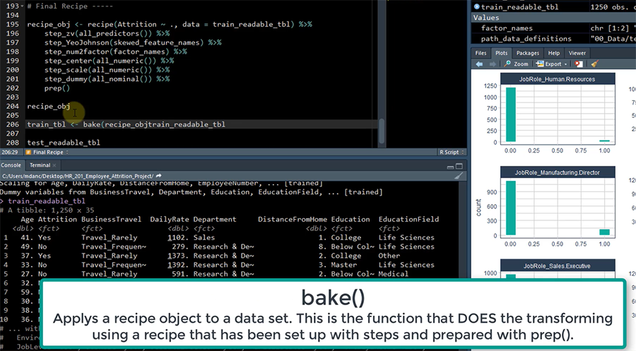
Next, I used bake() on the training and testing data sets to implement the minimal transformations.
x_train_processed_tbl <- bake(rec_obj, x_train_tbl)
x_test_processed_tbl  <- bake(rec_obj, x_test_tbl)
We can see the results of the transformation. For brevity, I show the first 30 columns and use the glimpse() function to quickly scan the data.
Before transformation (x_train_tbl), we can see that NA values are present and many of the flags are coded as integer.
# Before transformation
x_train_tbl %>%
    select(1:30) %>%
    glimpse()
## Observations: 307,511
## Variables: 30
## $ SK_ID_CURR                 <int> 100002, 100003, 100004, 100006...
## $ NAME_CONTRACT_TYPE         <chr> "Cash loans", "Cash loans", "R...
## $ CODE_GENDER                <chr> "M", "F", "M", "F", "M", "M", ...
## $ FLAG_OWN_CAR               <chr> "N", "N", "Y", "N", "N", "N", ...
## $ FLAG_OWN_REALTY            <chr> "Y", "N", "Y", "Y", "Y", "Y", ...
## $ CNT_CHILDREN               <int> 0, 0, 0, 0, 0, 0, 1, 0, 0, 0, ...
## $ AMT_INCOME_TOTAL           <dbl> 202500.00, 270000.00, 67500.00...
## $ AMT_CREDIT                 <dbl> 406597.5, 1293502.5, 135000.0,...
## $ AMT_ANNUITY                <dbl> 24700.5, 35698.5, 6750.0, 2968...
## $ AMT_GOODS_PRICE            <dbl> 351000, 1129500, 135000, 29700...
## $ NAME_TYPE_SUITE            <chr> "Unaccompanied", "Family", "Un...
## $ NAME_INCOME_TYPE           <chr> "Working", "State servant", "W...
## $ NAME_EDUCATION_TYPE        <chr> "Secondary / secondary special...
## $ NAME_FAMILY_STATUS         <chr> "Single / not married", "Marri...
## $ NAME_HOUSING_TYPE          <chr> "House / apartment", "House / ...
## $ REGION_POPULATION_RELATIVE <dbl> 0.018801, 0.003541, 0.010032, ...
## $ DAYS_BIRTH                 <int> -9461, -16765, -19046, -19005,...
## $ DAYS_EMPLOYED              <int> -637, -1188, -225, -3039, -303...
## $ DAYS_REGISTRATION          <dbl> -3648, -1186, -4260, -9833, -4...
## $ DAYS_ID_PUBLISH            <int> -2120, -291, -2531, -2437, -34...
## $ OWN_CAR_AGE                <dbl> NA, NA, 26, NA, NA, NA, 17, 8,...
## $ FLAG_MOBIL                 <int> 1, 1, 1, 1, 1, 1, 1, 1, 1, 1, ...
## $ FLAG_EMP_PHONE             <int> 1, 1, 1, 1, 1, 1, 1, 1, 0, 1, ...
## $ FLAG_WORK_PHONE            <int> 0, 0, 1, 0, 0, 1, 0, 1, 0, 0, ...
## $ FLAG_CONT_MOBILE           <int> 1, 1, 1, 1, 1, 1, 1, 1, 1, 1, ...
## $ FLAG_PHONE                 <int> 1, 1, 1, 0, 0, 1, 1, 0, 0, 0, ...
## $ FLAG_EMAIL                 <int> 0, 0, 0, 0, 0, 0, 0, 0, 0, 0, ...
## $ OCCUPATION_TYPE            <chr> "Laborers", "Core staff", "Lab...
## $ CNT_FAM_MEMBERS            <dbl> 1, 2, 1, 2, 1, 2, 3, 2, 2, 1, ...
## $ REGION_RATING_CLIENT       <int> 2, 1, 2, 2, 2, 2, 2, 3, 2, 2, ...
After the transformation (x_train_processed_tbl), the NA values are imputed, and we are left with factor and numeric (integer and double) data.
# After transformation
x_train_processed_tbl %>%
    select(1:30) %>%
    glimpse()
## Observations: 307,511
## Variables: 30
## $ SK_ID_CURR                 <int> 100002, 100003, 100004, 100006...
## $ NAME_CONTRACT_TYPE         <fct> Cash loans, Cash loans, Revolv...
## $ CODE_GENDER                <fct> M, F, M, F, M, M, F, M, F, M, ...
## $ FLAG_OWN_CAR               <fct> N, N, Y, N, N, N, Y, Y, N, N, ...
## $ FLAG_OWN_REALTY            <fct> Y, N, Y, Y, Y, Y, Y, Y, Y, Y, ...
## $ CNT_CHILDREN               <int> 0, 0, 0, 0, 0, 0, 1, 0, 0, 0, ...
## $ AMT_INCOME_TOTAL           <dbl> 202500.00, 270000.00, 67500.00...
## $ AMT_CREDIT                 <dbl> 406597.5, 1293502.5, 135000.0,...
## $ AMT_ANNUITY                <dbl> 24700.5, 35698.5, 6750.0, 2968...
## $ AMT_GOODS_PRICE            <dbl> 351000, 1129500, 135000, 29700...
## $ NAME_TYPE_SUITE            <fct> Unaccompanied, Family, Unaccom...
## $ NAME_INCOME_TYPE           <fct> Working, State servant, Workin...
## $ NAME_EDUCATION_TYPE        <fct> Secondary / secondary special,...
## $ NAME_FAMILY_STATUS         <fct> Single / not married, Married,...
## $ NAME_HOUSING_TYPE          <fct> House / apartment, House / apa...
## $ REGION_POPULATION_RELATIVE <dbl> 0.018801, 0.003541, 0.010032, ...
## $ DAYS_BIRTH                 <int> -9461, -16765, -19046, -19005,...
## $ DAYS_EMPLOYED              <int> -637, -1188, -225, -3039, -303...
## $ DAYS_REGISTRATION          <dbl> -3648, -1186, -4260, -9833, -4...
## $ DAYS_ID_PUBLISH            <int> -2120, -291, -2531, -2437, -34...
## $ OWN_CAR_AGE                <dbl> 12.06109, 12.06109, 26.00000, ...
## $ FLAG_MOBIL                 <fct> 1, 1, 1, 1, 1, 1, 1, 1, 1, 1, ...
## $ FLAG_EMP_PHONE             <fct> 1, 1, 1, 1, 1, 1, 1, 1, 0, 1, ...
## $ FLAG_WORK_PHONE            <fct> 0, 0, 1, 0, 0, 1, 0, 1, 0, 0, ...
## $ FLAG_CONT_MOBILE           <fct> 1, 1, 1, 1, 1, 1, 1, 1, 1, 1, ...
## $ FLAG_PHONE                 <fct> 1, 1, 1, 0, 0, 1, 1, 0, 0, 0, ...
## $ FLAG_EMAIL                 <fct> 0, 0, 0, 0, 0, 0, 0, 0, 0, 0, ...
## $ OCCUPATION_TYPE            <fct> Laborers, Core staff, Laborers...
## $ CNT_FAM_MEMBERS            <dbl> 1, 2, 1, 2, 1, 2, 3, 2, 2, 1, ...
## $ REGION_RATING_CLIENT       <fct> 2, 1, 2, 2, 2, 2, 2, 3, 2, 2, ...
I also converted the target to a factor, which is the format needed for H2O to perform binary classification. The trick is to convert the numeric value to character then to factor.
y_train_processed_tbl <- y_train_tbl %>%
    mutate(TARGET = TARGET %>% as.character() %>% as.factor())
Last, I removed the unprocessed datasets and recipe object to save memory.
rm(rec_obj)
rm(x_train_tbl)
rm(x_test_tbl)
rm(y_train_tbl)
Interested in Learning Preprocessing Strategies For Business?
If you're interested in learning how to apply the preprocessing strategies using R Programming beyond the simplified strategy shown, we teach preprocessing with recipes in Chapter 3 of Data Science For Business (DS4B 201-R) as part of our 10-Week end-to-end Employee Churn data science project.
Get Started Today!
Modeling
I implemented Automated Machine Learning (AutoML) with H2O. First, I loaded h2o and initialized a local cluster with h2o.init(). We can also supply h2o.no_progress() to eliminate progress bars.
h2o.init()
##  Connection successful!
##
## R is connected to the H2O cluster:
##     H2O cluster uptime:         4 hours 42 minutes
##     H2O cluster version:        3.16.0.2
##     H2O cluster version age:    8 months and 7 days !!!
##     H2O cluster name:           H2O_started_from_R_mdanc_inu316
##     H2O cluster total nodes:    1
##     H2O cluster total memory:   1.85 GB
##     H2O cluster total cores:    8
##     H2O cluster allowed cores:  8
##     H2O cluster healthy:        TRUE
##     H2O Connection ip:          localhost
##     H2O Connection port:        54321
##     H2O Connection proxy:       NA
##     H2O Internal Security:      FALSE
##     H2O API Extensions:         Algos, AutoML, Core V3, Core V4
##     R Version:                  R version 3.4.4 (2018-03-15)
h2o.no_progress()
Next, I converted the dataframe to an H2O Frame using as.h2o(). H2O expects both the target and the training features to be in the same data frame, so I used bind_cols() first.
data_h2o <- as.h2o(bind_cols(y_train_processed_tbl, x_train_processed_tbl))
I split the training data into train, validation, and test sets into a 70/15/15 split using h2o.splitFrame(). Note that I are only used the loan application training data and not the testing data for this part (the testing data will be used to make the Kaggle Competition submission).
splits_h2o <- h2o.splitFrame(data_h2o, ratios = c(0.7, 0.15), seed = 1234)

train_h2o <- splits_h2o[[1]]
valid_h2o <- splits_h2o[[2]]
test_h2o  <- splits_h2o[[3]]
Next, I ran h2o.automl(). I set max_runtime_secs = 90 to speed the training time up at the expense of some(default is 3600, which can take quite a while). The resulting leader model is produced in approximately 6 minutes.
y <- "TARGET"
x <- setdiff(names(train_h2o), y)

automl_models_h2o <- h2o.automl(
    x = x,
    y = y,
    training_frame    = train_h2o,
    validation_frame  = valid_h2o,
    leaderboard_frame = test_h2o,
    max_runtime_secs  = 90
)
automl_leader <- automl_models_h2o@leader
Interested in Learning H2O AutoML For Business?
If you're interested in learning how to perform H2O Automated Machine Learning using R Programming beyond the simplified modeling shown, we teach H2O AutoML modeling (including Grid Search and Cross Validation) in Chapter 4 of Data Science For Business (DS4B 201-R) as part of our 10-Week end-to-end Employee Churn data science project.
Get Started Today!
This part was excluded from the timed challenge since the model was developed and this is simply testing the validity of the results and submitting the final solution.
We can perform a brief performance analysis to assess the AutoML Leader model. First, let’s create an H2O performance object using h2o.performance(). We’ll set new data to test_h2o. Note that this is not the application test set, but rather a random sample of 15% of the application training set.
performance_h2o <- h2o.performance(automl_leader, newdata = test_h2o)
Next, let’s output the Confusion Matrix using the h2o.confusionMatrix() function. It’s important to understand that this model uses a threshold of 0.139, which maximizes the F1. This is NOT always the best case for the business. If you want to learn how to optimize the classification threshold, our Data Science For Business With R course covers Expected Value, Threshold Optimization, and Sensitivity Analysis in Chapters 7 and 8.
performance_h2o %>%
    h2o.confusionMatrix()
## Confusion Matrix (vertical: actual; across: predicted)  for max f1 @ threshold = 0.112512548039536:
##            0    1    Error         Rate
## 0      36871 5516 0.130134  =5516/42387
## 1       2185 1528 0.588473   =2185/3713
## Totals 39056 7044 0.167050  =7701/46100
We can see that 1528 people that defaulted were correctly detected, 5516 were incorrectly predicted to be default but actually did not, and 2185 were incorrectly predicted to not default, but actually did. This last group is called False Negatives, and this population can be EXTREMELY COSTLY to the lender. Typically a lot more costly than False Positives. This is why threshold optimization is important. Check out DS4B 201-R if you want to learn how to do threshold optimization.
We can also check out the AUC on the performance set. We’re getting about 0.73, which is pretty good.
performance_h2o %>%
    h2o.auc()
## [1] 0.7330787
Interested in Learning H2O Performance Analysis For Business?
If you're interested in learning how to do performance analysis for H2O modeling using R Programming beyond the simplified performance analysis shown, we teach:
- Chapter 5: H2O Performance Analysis (ROC, Precision vs Recall, Gain & Lift) on an entire leaderboard of H2O models (stacked ensembles, deep learning, random forest, and more)
- Chapter 7: Expected Value Framework and targeting using cost/benefit analysis
- Chapter 8: Optimizing the threshold to maximize profitability and performing sensitivity analysis to account for unknowns.
Check out Data Science For Business (DS4B 201-R) as part of our 10-Week end-to-end Employee Churn data science project.
Get Started Today!
Kaggle Competition Submission
This is the moment of truth. I made my final predictions for the Kaggle Competition. Here’s the procedure and final results.
First, we can make some predictions using h2o.predict().
prediction_h2o <- h2o.predict(automl_leader, newdata = as.h2o(x_test_processed_tbl))
Next, let’s convert to a tibble and bind with the correct SK_ID_CURR. We’ll grab the SK_ID_CURR and p1 (positive class probability) columns, which is the format expected for the Kaggle Competition.
prediction_tbl <- prediction_h2o %>%
    as.tibble() %>%
    bind_cols(
        x_test_processed_tbl %>% select(SK_ID_CURR)
    ) %>%
    select(SK_ID_CURR, p1) %>%
    rename(TARGET = p1)

prediction_tbl
## # A tibble: 48,744 x 2
##    SK_ID_CURR TARGET
##         <int>  <dbl>
##  1     100001 0.0632
##  2     100005 0.0969
##  3     100013 0.0516
##  4     100028 0.0418
##  5     100038 0.0892
##  6     100042 0.0477
##  7     100057 0.0367
##  8     100065 0.0613
##  9     100066 0.0348
## 10     100067 0.131
## # ... with 48,734 more rows
Finally, we can output the submission to a CSV file using the write_csv() function.
prediction_tbl %>%
    write_csv(path = "submission_001.csv")
Submitting my results, I got an AUC of approximately 0.70. Not bad for 30 minutes of modeling.
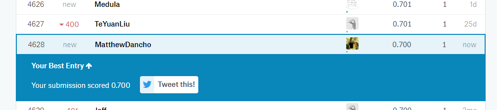
Kaggle Submission
The important thing to understand is that this is a great baseline for a model. We can begin to improve it, which can take significant effort depending on how far you want to go.
We did not perform feature engineering and any additional model tuning beyond what AutoML performs by default. Doing so will get us closer to the top results.
Next Steps (Transform Your Abilities)
It’s critical to understand that modeling is just one part of the overall data science project. Don’t mistake - it’s an important part, but other parts are equally if not more important, which is why our Data Science For Business With R (DS4B 201-R) course is successfully teaching data science students how to apply data science in the real world.
We teach end-to-end data science. This means you learn how to:
-
Chapter 1: Sizing The Problem, Custom Functions With Tidy Eval: Learn how to understand if a business problem exists by sizing the problem. In addition, create custom functions using Tidy Eval, a programming interface that is needed if you want to build custom functions using dplyr, ggplot2.
-
Chapter 2: Exploration with GGally, skimr - We show you how to explore data and identify relationships efficiently and effectively
-
Chapter 3: recipes, Premodeling Correlation Analysis: We teach you how to use recipes to develop data transformation workflow and we show you how to perform a pre-modeling correlation analysis so you do not move into modeling prematurely, which again saves you time
-
Chapters 4 and 5: H2O AutoML: You will first learn how to use all of the major h2o functions to perform automated machine learning for binary classification including working with the H2O leaderboard, visualizing results, and performing grid search and cross validation. In the next chapter, you learn how to evaluate multiple models against each other with ROC, Precision vs Recall, Gain and Lift, which is necessary to explain your choices for best model to the business stakeholders (your manager and key decision makers).
-
Chapter 6: LIME: You learn how to create local explanations to interpret black-box machine learning models. Explanations for the model predictions are critical because the business cannot do anything to improve unless they understand why. We show you how with lime.
-
Chapters 7 and 8: Expected Value Framework, Threshold Optimization, Sensitivity Analysis: These are my two favorite chapters because they show you how to link the churn classification model to financial results, and they teach purrr for iterative grid-search style optimization! These are POWERFUL CONCEPTS.
-
Chapter 9: Recommendation Algorithm: We again use a correlation analysis but in a different way. We discretize, creating a special visualization that enables us to develop a recommendation strategy.
Data Science For Business With R (DS4B 201-R)
Learn everything you need to know to complete a real-world, end-to-end data science project with the R programming language. Transform your abilities in 10 weeks.
Get Started Today!
Business Science University Course Roadmap
We have one course out and two courses coming soon!
Data Science For Business With R (DS4B 201-R)
Over the course of 10 weeks, we teach you how to solve an end-to-end data science project. Available now!
Transform you abilities by solving employee churn over a 10-week end-to-end data science project in DS4B 201-R
Get Started Today!
Building A Shiny Application (DS4B 301-R)
Our next course teaches you how to take the H2O Model, LIME explanation results, and the recommendation algorithm you develop in DS4B 201-R and turn it into a Shiny Web Application that predicts employee attrition! Coming in Q3 2018.
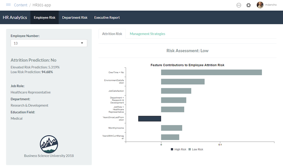
Shiny App That Predicts Attrition and Recommends Management Strategies, Taught in DS4B 301-R (Building A Shiny Web App)
Kelly O’Briant is lead developer for the Shiny App Course coming soon. She’s a brilliant software engineer / data scientist that knows how to make a great looking and performing Shiny app.
Sign Up! Coming Q3!
Data Science For Business With Python (DS4B 201-P)
Did we mention with have a DS4B Python Course coming?!?! Well we do! Coming in Q4 2018.
The problem changes: Customer Churn! The tools will be H2O, LIME, and a host of other tools implemented in Python + Spark.
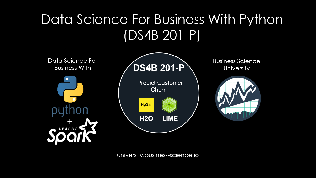
Python Track: Data Science For Business With Python And Spark
Favio Vazquez, Principle Data Scientist at OXXO, is building the Python + Spark equivalent of DS4B 201-R. He’s so talented knowing Python, Spark, and R, along with a host of other data science tools.
Sign Up! Coming Q4!
Don’t Miss A Beat
Connect With Business Science
If you like our software (anomalize, tidyquant, tibbletime, timetk, and sweep), our courses, and our company, you can connect with us: