HR Analytics: Using Machine Learning to Predict Employee Turnover
Written by Matt Dancho
Employee turnover (attrition) is a major cost to an organization, and predicting turnover is at the forefront of needs of Human Resources (HR) in many organizations. Until now the mainstream approach has been to use logistic regression or survival curves to model employee attrition. However, with advancements in machine learning (ML), we can now get both better predictive performance and better explanations of what critical features are linked to employee attrition. In this post, we’ll use two cutting edge techniques. First, we’ll use the h2o package’s new FREE automatic machine learning algorithm, h2o.automl(), to develop a predictive model that is in the same ballpark as commercial products in terms of ML accuracy. Then we’ll use the new lime package that enables breakdown of complex, black-box machine learning models into variable importance plots. We can’t stress how excited we are to share this post because it’s a much needed step towards machine learning in business applications!!! Enjoy.
Employee Attrition: A Major Problem
Bill Gates was once quoted as saying,
“You take away our top 20 employees and we [Microsoft] become a mediocre company”.
His statement cuts to the core of a major problem: employee attrition. An organization is only as good as its employees, and these people are the true source of its competitive advantage.
Organizations face huge costs resulting from employee turnover. Some costs are tangible such as training expenses and the time it takes from when an employee starts to when they become a productive member. However, the most important costs are intangible. Consider what’s lost when a productive employee quits: new product ideas, great project management, or customer relationships.
With advances in machine learning and data science, its possible to not only predict employee attrition but to understand the key variables that influence turnover. We’ll take a look at two cutting edge techniques:
-
Machine Learning with h2o.automl() from the h2o package: This function takes automated machine learning to the next level by testing a number of advanced algorithms such as random forests, ensemble methods, and deep learning along with more traditional algorithms such as logistic regression. The main takeaway is that we can now easily achieve predictive performance that is in the same ball park (and in some cases even better than) commercial algorithms and ML/AI software.
-
Feature Importance with the lime package: The problem with advanced machine learning algorithms such as deep learning is that it’s near impossible to understand the algorithm because of its complexity. This has all changed with the lime package. The major advancement with lime is that, by recursively analyzing the models locally, it can extract feature importance that repeats globally. What this means to us is that lime has opened the door to understanding the ML models regardless of complexity. Now the best (and typically very complex) models can also be investigated and potentially understood as to what variables or features make the model tick.
Employee Attrition: Machine Learning Analysis
With these new automated ML tools combined with tools to uncover critical variables, we now have capabilities for both extreme predictive accuracy and understandability, which was previously impossible! We’ll investigate an HR Analytic example of employee attrition that was evaluated by IBM Watson.
IBM Watson (Where we got the data)
The example comes from IBM Watson Analytics website. You can download the data and read the analysis here:
To summarize, the article makes a usage case for IBM Watson as an automated ML platform. The article shows that using Watson, the analyst was able to detect features that led to increased probability of attrition.
Automated Machine Learning (What we did with the data)
In this example we’ll show how we can use the combination of H2O for developing a complex model with high predictive accuracy on unseen data and then how we can use LIME to understand important features related to employee attrition.
Packages
Load the following packages.
# Load the following packages
library(tidyquant)  # Loads tidyverse and several other pkgs
library(readxl)     # Super simple excel reader
library(h2o)        # Professional grade ML pkg
library(lime)       # Explain complex black-box ML models
Data
Download the data here. You can load the data using read_excel(), pointing the path to your local file.
# Read excel data
hr_data_raw <- read_excel(path = "data/WA_Fn-UseC_-HR-Employee-Attrition.xlsx")
Let’s check out the raw data. It’s 1470 rows (observations) by 35 columns (features). The “Attrition” column is our target. We’ll use all other columns as features to our model.
# View first 10 rows
hr_data_raw[1:10,] %>%
    knitr::kable(caption = "First 10 rows")
| Age |
Attrition |
BusinessTravel |
DailyRate |
Department |
DistanceFromHome |
Education |
EducationField |
EmployeeCount |
EmployeeNumber |
EnvironmentSatisfaction |
Gender |
HourlyRate |
JobInvolvement |
JobLevel |
JobRole |
JobSatisfaction |
MaritalStatus |
MonthlyIncome |
MonthlyRate |
NumCompaniesWorked |
Over18 |
OverTime |
PercentSalaryHike |
PerformanceRating |
RelationshipSatisfaction |
StandardHours |
StockOptionLevel |
TotalWorkingYears |
TrainingTimesLastYear |
WorkLifeBalance |
YearsAtCompany |
YearsInCurrentRole |
YearsSinceLastPromotion |
YearsWithCurrManager |
| 41 |
Yes |
Travel_Rarely |
1102 |
Sales |
1 |
2 |
Life Sciences |
1 |
1 |
2 |
Female |
94 |
3 |
2 |
Sales Executive |
4 |
Single |
5993 |
19479 |
8 |
Y |
Yes |
11 |
3 |
1 |
80 |
0 |
8 |
0 |
1 |
6 |
4 |
0 |
5 |
| 49 |
No |
Travel_Frequently |
279 |
Research & Development |
8 |
1 |
Life Sciences |
1 |
2 |
3 |
Male |
61 |
2 |
2 |
Research Scientist |
2 |
Married |
5130 |
24907 |
1 |
Y |
No |
23 |
4 |
4 |
80 |
1 |
10 |
3 |
3 |
10 |
7 |
1 |
7 |
| 37 |
Yes |
Travel_Rarely |
1373 |
Research & Development |
2 |
2 |
Other |
1 |
4 |
4 |
Male |
92 |
2 |
1 |
Laboratory Technician |
3 |
Single |
2090 |
2396 |
6 |
Y |
Yes |
15 |
3 |
2 |
80 |
0 |
7 |
3 |
3 |
0 |
0 |
0 |
0 |
| 33 |
No |
Travel_Frequently |
1392 |
Research & Development |
3 |
4 |
Life Sciences |
1 |
5 |
4 |
Female |
56 |
3 |
1 |
Research Scientist |
3 |
Married |
2909 |
23159 |
1 |
Y |
Yes |
11 |
3 |
3 |
80 |
0 |
8 |
3 |
3 |
8 |
7 |
3 |
0 |
| 27 |
No |
Travel_Rarely |
591 |
Research & Development |
2 |
1 |
Medical |
1 |
7 |
1 |
Male |
40 |
3 |
1 |
Laboratory Technician |
2 |
Married |
3468 |
16632 |
9 |
Y |
No |
12 |
3 |
4 |
80 |
1 |
6 |
3 |
3 |
2 |
2 |
2 |
2 |
| 32 |
No |
Travel_Frequently |
1005 |
Research & Development |
2 |
2 |
Life Sciences |
1 |
8 |
4 |
Male |
79 |
3 |
1 |
Laboratory Technician |
4 |
Single |
3068 |
11864 |
0 |
Y |
No |
13 |
3 |
3 |
80 |
0 |
8 |
2 |
2 |
7 |
7 |
3 |
6 |
| 59 |
No |
Travel_Rarely |
1324 |
Research & Development |
3 |
3 |
Medical |
1 |
10 |
3 |
Female |
81 |
4 |
1 |
Laboratory Technician |
1 |
Married |
2670 |
9964 |
4 |
Y |
Yes |
20 |
4 |
1 |
80 |
3 |
12 |
3 |
2 |
1 |
0 |
0 |
0 |
| 30 |
No |
Travel_Rarely |
1358 |
Research & Development |
24 |
1 |
Life Sciences |
1 |
11 |
4 |
Male |
67 |
3 |
1 |
Laboratory Technician |
3 |
Divorced |
2693 |
13335 |
1 |
Y |
No |
22 |
4 |
2 |
80 |
1 |
1 |
2 |
3 |
1 |
0 |
0 |
0 |
| 38 |
No |
Travel_Frequently |
216 |
Research & Development |
23 |
3 |
Life Sciences |
1 |
12 |
4 |
Male |
44 |
2 |
3 |
Manufacturing Director |
3 |
Single |
9526 |
8787 |
0 |
Y |
No |
21 |
4 |
2 |
80 |
0 |
10 |
2 |
3 |
9 |
7 |
1 |
8 |
| 36 |
No |
Travel_Rarely |
1299 |
Research & Development |
27 |
3 |
Medical |
1 |
13 |
3 |
Male |
94 |
3 |
2 |
Healthcare Representative |
3 |
Married |
5237 |
16577 |
6 |
Y |
No |
13 |
3 |
2 |
80 |
2 |
17 |
3 |
2 |
7 |
7 |
7 |
7 |
The only pre-processing we’ll do in this example is change all character data types to factors. This is needed for H2O. We could make a number of other numeric data that is actually categorical factors, but this tends to increase modeling time and can have little improvement on model performance.
hr_data <- hr_data_raw %>%
    mutate_if(is.character, as.factor) %>%
    select(Attrition, everything())
Let’s take a glimpse at the processed dataset. We can see all of the columns. Note our target (“Attrition”) is the first column.
glimpse(hr_data)
## Observations: 1,470
## Variables: 35
## $ Attrition                <fctr> Yes, No, Yes, No, No, No, No, N...
## $ Age                      <dbl> 41, 49, 37, 33, 27, 32, 59, 30, ...
## $ BusinessTravel           <fctr> Travel_Rarely, Travel_Frequentl...
## $ DailyRate                <dbl> 1102, 279, 1373, 1392, 591, 1005...
## $ Department               <fctr> Sales, Research & Development, ...
## $ DistanceFromHome         <dbl> 1, 8, 2, 3, 2, 2, 3, 24, 23, 27,...
## $ Education                <dbl> 2, 1, 2, 4, 1, 2, 3, 1, 3, 3, 3,...
## $ EducationField           <fctr> Life Sciences, Life Sciences, O...
## $ EmployeeCount            <dbl> 1, 1, 1, 1, 1, 1, 1, 1, 1, 1, 1,...
## $ EmployeeNumber           <dbl> 1, 2, 4, 5, 7, 8, 10, 11, 12, 13...
## $ EnvironmentSatisfaction  <dbl> 2, 3, 4, 4, 1, 4, 3, 4, 4, 3, 1,...
## $ Gender                   <fctr> Female, Male, Male, Female, Mal...
## $ HourlyRate               <dbl> 94, 61, 92, 56, 40, 79, 81, 67, ...
## $ JobInvolvement           <dbl> 3, 2, 2, 3, 3, 3, 4, 3, 2, 3, 4,...
## $ JobLevel                 <dbl> 2, 2, 1, 1, 1, 1, 1, 1, 3, 2, 1,...
## $ JobRole                  <fctr> Sales Executive, Research Scien...
## $ JobSatisfaction          <dbl> 4, 2, 3, 3, 2, 4, 1, 3, 3, 3, 2,...
## $ MaritalStatus            <fctr> Single, Married, Single, Marrie...
## $ MonthlyIncome            <dbl> 5993, 5130, 2090, 2909, 3468, 30...
## $ MonthlyRate              <dbl> 19479, 24907, 2396, 23159, 16632...
## $ NumCompaniesWorked       <dbl> 8, 1, 6, 1, 9, 0, 4, 1, 0, 6, 0,...
## $ Over18                   <fctr> Y, Y, Y, Y, Y, Y, Y, Y, Y, Y, Y...
## $ OverTime                 <fctr> Yes, No, Yes, Yes, No, No, Yes,...
## $ PercentSalaryHike        <dbl> 11, 23, 15, 11, 12, 13, 20, 22, ...
## $ PerformanceRating        <dbl> 3, 4, 3, 3, 3, 3, 4, 4, 4, 3, 3,...
## $ RelationshipSatisfaction <dbl> 1, 4, 2, 3, 4, 3, 1, 2, 2, 2, 3,...
## $ StandardHours            <dbl> 80, 80, 80, 80, 80, 80, 80, 80, ...
## $ StockOptionLevel         <dbl> 0, 1, 0, 0, 1, 0, 3, 1, 0, 2, 1,...
## $ TotalWorkingYears        <dbl> 8, 10, 7, 8, 6, 8, 12, 1, 10, 17...
## $ TrainingTimesLastYear    <dbl> 0, 3, 3, 3, 3, 2, 3, 2, 2, 3, 5,...
## $ WorkLifeBalance          <dbl> 1, 3, 3, 3, 3, 2, 2, 3, 3, 2, 3,...
## $ YearsAtCompany           <dbl> 6, 10, 0, 8, 2, 7, 1, 1, 9, 7, 5...
## $ YearsInCurrentRole       <dbl> 4, 7, 0, 7, 2, 7, 0, 0, 7, 7, 4,...
## $ YearsSinceLastPromotion  <dbl> 0, 1, 0, 3, 2, 3, 0, 0, 1, 7, 0,...
## $ YearsWithCurrManager     <dbl> 5, 7, 0, 0, 2, 6, 0, 0, 8, 7, 3,...
Modeling Employee Attrition
We are going to use the h2o.automl() function from the H2O platform to model employee attrition.
H2O
First, we need to initialize the Java Virtual Machine (JVM) that H2O uses locally.
# Initialize H2O JVM
h2o.init()
##
## H2O is not running yet, starting it now...
##
## Note:  In case of errors look at the following log files:
##     C:\Users\mdanc\AppData\Local\Temp\RtmpMdwBB4/h2o_mdanc_started_from_r.out
##     C:\Users\mdanc\AppData\Local\Temp\RtmpMdwBB4/h2o_mdanc_started_from_r.err
##
##
## Starting H2O JVM and connecting: . Connection successful!
##
## R is connected to the H2O cluster:
##     H2O cluster uptime:         2 seconds 524 milliseconds
##     H2O cluster version:        3.15.0.4004
##     H2O cluster version age:    28 days, 20 hours and 35 minutes
##     H2O cluster name:           H2O_started_from_R_mdanc_pul628
##     H2O cluster total nodes:    1
##     H2O cluster total memory:   3.52 GB
##     H2O cluster total cores:    8
##     H2O cluster allowed cores:  8
##     H2O cluster healthy:        TRUE
##     H2O Connection ip:          localhost
##     H2O Connection port:        54321
##     H2O Connection proxy:       NA
##     H2O Internal Security:      FALSE
##     H2O API Extensions:         Algos, AutoML, Core V3, Core V4
##     R Version:                  R version 3.4.0 (2017-04-21)
h2o.no_progress() # Turn off output of progress bars
Next, we change our data to an h2o object that the package can interpret. We also split the data into training, validation, and test sets. Our preference is to use 70%, 15%, 15%, respectively.
# Split data into Train/Validation/Test Sets
hr_data_h2o <- as.h2o(hr_data)

split_h2o <- h2o.splitFrame(hr_data_h2o, c(0.7, 0.15), seed = 1234 )

train_h2o <- h2o.assign(split_h2o[[1]], "train" ) # 70%
valid_h2o <- h2o.assign(split_h2o[[2]], "valid" ) # 15%
test_h2o  <- h2o.assign(split_h2o[[3]], "test" )  # 15%
Model
Now we are ready to model. We’ll set the target and feature names. The target is what we aim to predict (in our case “Attrition”). The features (every other column) are what we will use to model the prediction.
# Set names for h2o
y <- "Attrition"
x <- setdiff(names(train_h2o), y)
Now the fun begins. We run the h2o.automl() setting the arguments it needs to run models against. For more information, see the h2o.automl documentation.
x = x: The names of our feature columns.y = y: The name of our target column.training_frame = train_h2o: Our training set consisting of 70% of the data.leaderboard_frame = valid_h2o: Our validation set consisting of 15% of the data. H2O uses this to ensure the model does not overfit the data.max_runtime_secs = 30: We supply this to speed up H2O’s modeling. The algorithm has a large number of complex models so we want to keep things moving at the expense of some accuracy.
# Run the automated machine learning
automl_models_h2o <- h2o.automl(
    x = x,
    y = y,
    training_frame    = train_h2o,
    leaderboard_frame = valid_h2o,
    max_runtime_secs  = 30
    )
All of the models are stored the automl_models_h2o object. However, we are only concerned with the leader, which is the best model in terms of accuracy on the validation set. We’ll extract it from the models object.
# Extract leader model
automl_leader <- automl_models_h2o@leader
Predict
Now we are ready to predict on our test set, which is unseen from during our modeling process. This is the true test of performance. We use the h2o.predict() function to make predictions.
# Predict on hold-out set, test_h2o
pred_h2o <- h2o.predict(object = automl_leader, newdata = test_h2o)
Now we can evaluate our leader model. We’ll reformat the test set an add the predictions as column so we have the actual and prediction columns side-by-side.
# Prep for performance assessment
test_performance <- test_h2o %>%
    tibble::as_tibble() %>%
    select(Attrition) %>%
    add_column(pred = as.vector(pred_h2o$predict)) %>%
    mutate_if(is.character, as.factor)
test_performance
## # A tibble: 211 x 2
##    Attrition   pred
##       <fctr> <fctr>
##  1        No     No
##  2        No     No
##  3       Yes    Yes
##  4        No     No
##  5        No     No
##  6        No     No
##  7       Yes    Yes
##  8        No     No
##  9        No     No
## 10       Yes     No
## # ... with 201 more rows
We can use the table() function to quickly get a confusion table of the results. We see that the leader model wasn’t perfect, but it did a decent job identifying employees that are likely to quit. For perspective, a logistic regression would not perform nearly this well.
# Confusion table counts
confusion_matrix <- test_performance %>%
    table()
confusion_matrix
##          pred
## Attrition  No Yes
##       No  167  15
##       Yes  11  18
We’ll run through a binary classification analysis to understand the model performance.
# Performance analysis
tn <- confusion_matrix[1]
tp <- confusion_matrix[4]
fp <- confusion_matrix[3]
fn <- confusion_matrix[2]

accuracy <- (tp + tn) / (tp + tn + fp + fn)
misclassification_rate <- 1 - accuracy
recall <- tp / (tp + fn)
precision <- tp / (tp + fp)
null_error_rate <- tn / (tp + tn + fp + fn)

tibble(
    accuracy,
    misclassification_rate,
    recall,
    precision,
    null_error_rate
) %>%
    transpose()
## [[1]]
## [[1]]$accuracy
## [1] 0.8767773
##
## [[1]]$misclassification_rate
## [1] 0.1232227
##
## [[1]]$recall
## [1] 0.6206897
##
## [[1]]$precision
## [1] 0.5454545
##
## [[1]]$null_error_rate
## [1] 0.7914692
It is important to understand is that the accuracy can be misleading: 88% sounds pretty good especially for modeling HR data, but if we just pick Attrition = NO we would get an accuracy of about 79%. Doesn’t sound so great now.
Before we make our final judgement, let’s dive a little deeper into precision and recall. Precision is when the model predicts yes, how often is it actually yes. Recall (also true positive rate or specificity) is when the actual value is yes how often is the model correct. Confused yet? Let’s explain in terms of what’s important to HR.
Most HR groups would probably prefer to incorrectly classify folks not looking to quit as high potential of quiting rather than classify those that are likely to quit as not at risk. Because it’s important to not miss at risk employees, HR will really care about recall or when the actual value is Attrition = YES how often the model predicts YES.
Recall for our model is 62%. In an HR context, this is 62% more employees that could potentially be targeted prior to quiting. From that standpoint, an organization that loses 100 people per year could possibly target 62 implementing measures to retain.
LIME
We have a very good model that is capable of making very accurate predictions on unseen data, but what can it tell us about what causes attrition? Let’s find out using LIME.
Setup
The lime package implements LIME in R. One thing to note is that it’s not setup out-of-the-box to work with h2o. The good news is with a few functions we can get everything working properly. We’ll need to make two custom functions:
-
model_type: Used to tell lime what type of model we are dealing with. It could be classification, regression, survival, etc.
-
predict_model: Used to allow lime to perform predictions that its algorithm can interpret.
The first thing we need to do is identify the class of our model leader object. We do this with the class() function.
class(automl_leader)
## [1] "H2OBinomialModel"
## attr(,"package")
## [1] "h2o"
Next we create our model_type function. It’s only input is x the h2o model. The function simply returns “classification”, which tells LIME we are classifying.
# Setup lime::model_type() function for h2o
model_type.H2OBinomialModel <- function(x, ...) {
    # Function tells lime() what model type we are dealing with
    # 'classification', 'regression', 'survival', 'clustering', 'multilabel', etc
    #
    # x is our h2o model

    return("classification")
}
Now we can create our predict_model function. The trick here is to realize that it’s inputs must be x a model, newdata a dataframe object (this is important), and type which is not used but can be use to switch the output type. The output is also a little tricky because it must be in the format of probabilities by classification (this is important; shown next). Internally we just call the h2o.predict() function.
# Setup lime::predict_model() function for h2o
predict_model.H2OBinomialModel <- function(x, newdata, type, ...) {
    # Function performs prediction and returns dataframe with Response
    #
    # x is h2o model
    # newdata is data frame
    # type is only setup for data frame

    pred <- h2o.predict(x, as.h2o(newdata))

    # return probs
    return(as.data.frame(pred[,-1]))

}
Run this next script to show you what the output looks like and to test our predict_model function. See how it’s the probabilities by classification. It must be in this form for model_type = “classification”.
# Test our predict_model() function
predict_model(x = automl_leader, newdata = as.data.frame(test_h2o[,-1]), type = 'raw') %>%
    tibble::as_tibble()
## # A tibble: 211 x 2
##           No        Yes
##        <dbl>      <dbl>
##  1 0.7773040 0.22269598
##  2 0.9394525 0.06054745
##  3 0.0388503 0.96114970
##  4 0.9652307 0.03476933
##  5 0.8912266 0.10877342
##  6 0.9650042 0.03499577
##  7 0.1404600 0.85953998
##  8 0.9616790 0.03832103
##  9 0.8349220 0.16507804
## 10 0.6965064 0.30349364
## # ... with 201 more rows
Now the fun part, we create an explainer using the lime() function. Just pass the training data set without the “Attribution column”. The form must be a data frame, which is OK since our predict_model function will switch it to an h2o object. Set model = automl_leader our leader model, and bin_continuous = FALSE. We could tell the algorithm to bin continuous variables, but this may not make sense for categorical numeric data that we didn’t change to factors.
# Run lime() on training set
explainer <- lime::lime(
    as.data.frame(train_h2o[,-1]),
    model          = automl_leader,
    bin_continuous = FALSE)
Now we run the explain() function, which returns our explanation. This can take a minute to run so we limit it to just the first ten rows of the test data set. We set n_labels = 1 because we care about explaining a single class. Setting n_features = 4 returns the top four features that are critical to each case. Finally, setting kernel_width = 0.5 allows us to increase the “model_r2” value by shrinking the localized evaluation.
# Run explain() on explainer
explanation <- lime::explain(
    as.data.frame(test_h2o[1:10,-1]),
    explainer    = explainer,
    n_labels     = 1,
    n_features   = 4,
    kernel_width = 0.5)
Feature Importance Visualization
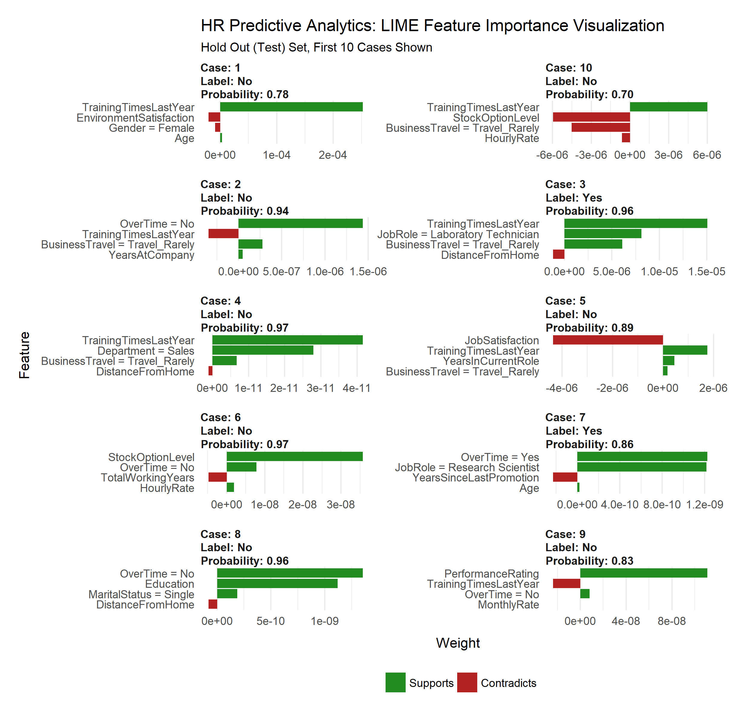
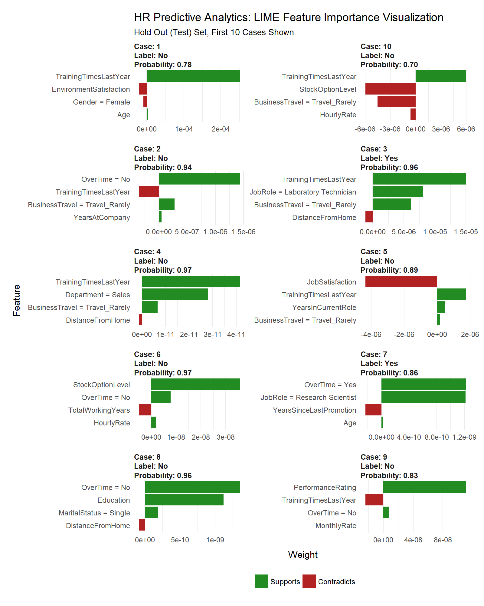
The payoff for the work we put in using LIME is this feature importance plot. This allows us to visualize each of the ten cases (observations) from the test data. The top four features for each case are shown. Note that they are not the same for each case. The green bars mean that the feature supports the model conclusion, and the red bars contradict. We’ll focus in on Cases with Label = Yes, which are predicted to have attrition. We can see a common theme with Case 3 and Case 7: Training Time, Job Role, and Over Time are among the top factors influencing attrition. These are only two cases, but they can be used to potentially generalize to the larger population as we will see next.
plot_features(explanation) +
    labs(title = "HR Predictive Analytics: LIME Feature Importance Visualization",
         subtitle = "Hold Out (Test) Set, First 10 Cases Shown")
What Features Are Linked To Employee Attrition?
Now we turn to our three critical features from the LIME Feature Importance Plot:
- Training Time
- Job Role
- Over Time
We’ll subset this data and visualize to detect trends.
# Focus on critical features of attrition
attrition_critical_features <- hr_data %>%
    tibble::as_tibble() %>%
    select(Attrition, TrainingTimesLastYear, JobRole, OverTime) %>%
    rowid_to_column(var = "Case")
attrition_critical_features
## # A tibble: 1,470 x 5
##     Case Attrition TrainingTimesLastYear                   JobRole
##    <int>    <fctr>                 <dbl>                    <fctr>
##  1     1       Yes                     0           Sales Executive
##  2     2        No                     3        Research Scientist
##  3     3       Yes                     3     Laboratory Technician
##  4     4        No                     3        Research Scientist
##  5     5        No                     3     Laboratory Technician
##  6     6        No                     2     Laboratory Technician
##  7     7        No                     3     Laboratory Technician
##  8     8        No                     2     Laboratory Technician
##  9     9        No                     2    Manufacturing Director
## 10    10        No                     3 Healthcare Representative
## # ... with 1,460 more rows, and 1 more variables: OverTime <fctr>
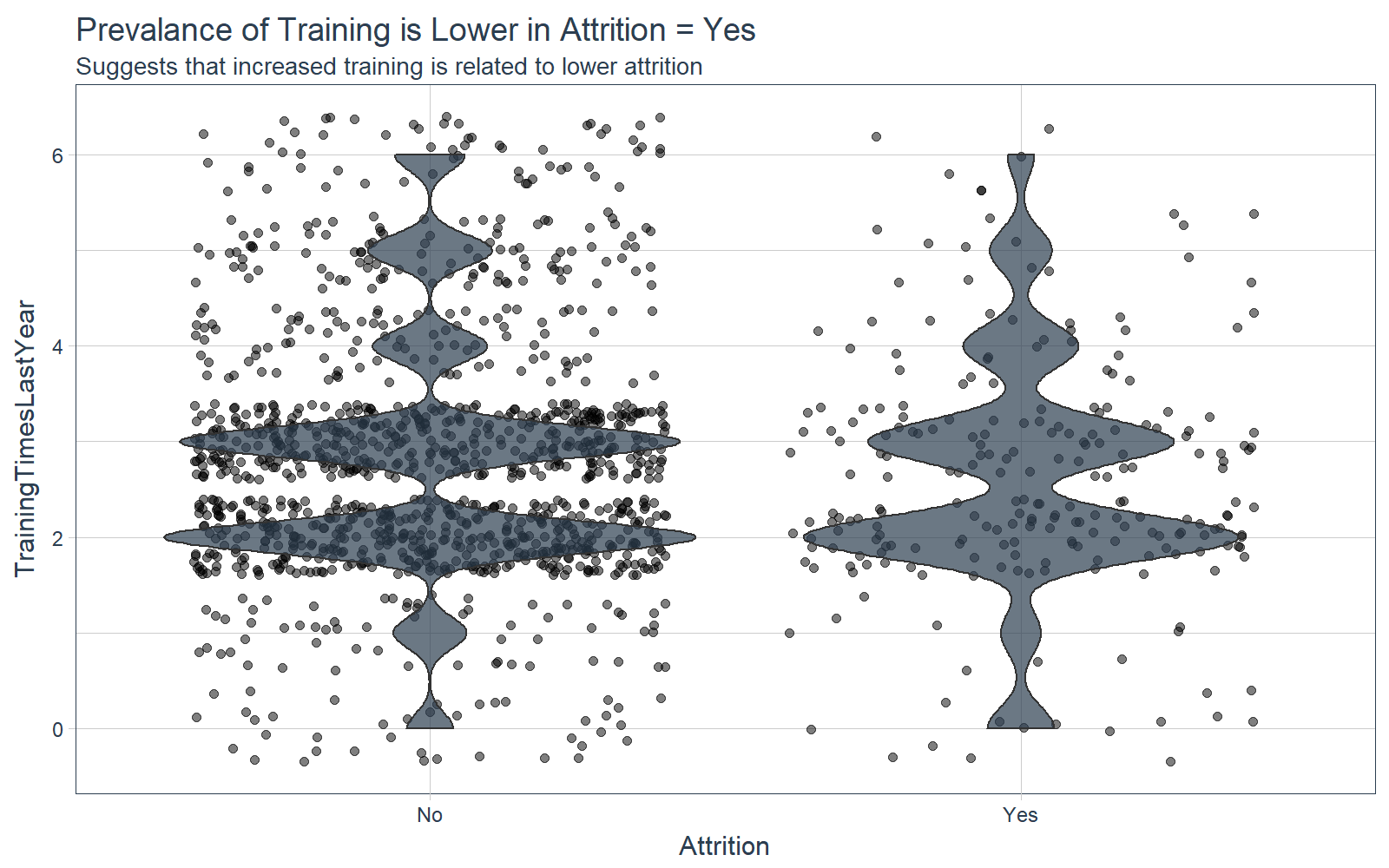
Training
From the violin plot, the employees that stay tend to have a large peaks at two and three trainings per year whereas the employees that leave tend to have a large peak at two trainings per year. This suggests that employees with more trainings may be less likely to leave.
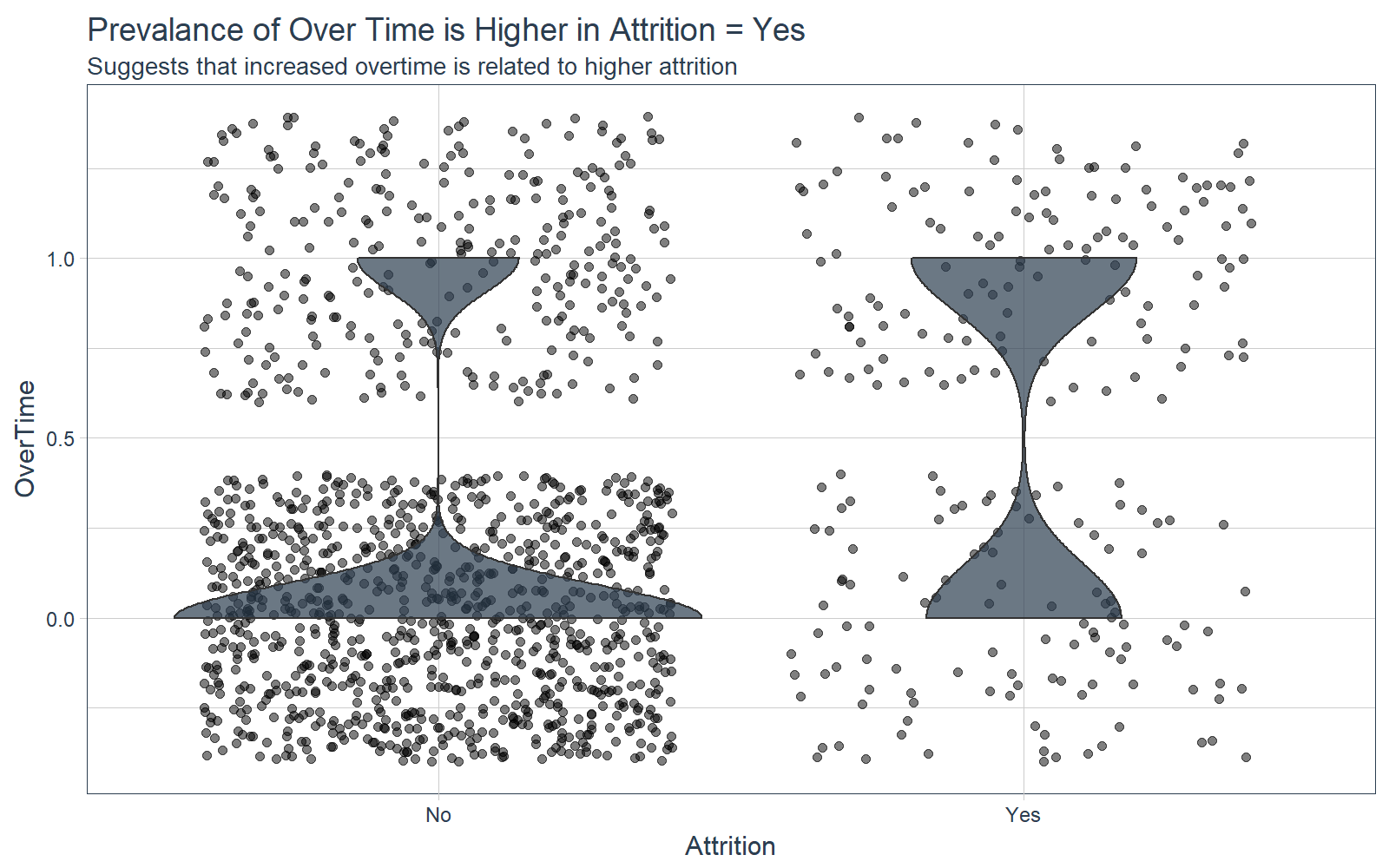
Overtime
The plot below shows a very interesting relationship: a very high proportion of employees that turnover are working over time. The opposite is true for employees that stay.
Job Role
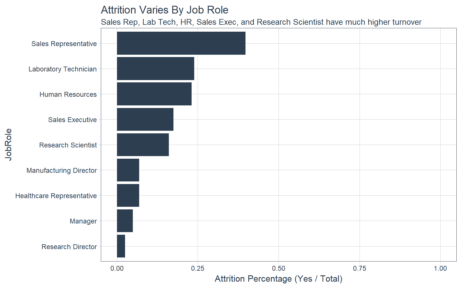
Several job roles are experiencing more turnover. Sales reps have the highest turnover at about 40% followed by Lab Technician, Human Resources, Sales Executive, and Research Scientist. It may be worthwhile to investigate what localized issues could be creating the high turnover among these groups within the organization.
Conclusions
There’s a lot to take away from this article. We showed how you can use predictive analytics to develop sophisticated models that very accurately detect employees that are at risk of turnover. The autoML algorithm from H2O.ai worked well for classifying attrition with an accuracy around 87% on unseen / unmodeled data. We then used LIME to breakdown the complex ensemble model returned from H2O into critical features that are related to attrition. Overall, this is a really useful example where we can see how machine learning and data science can be used in business applications.
Business Science University
Enjoy data science for business? We do too. This is why we created Business Science University where we teach you how to do Data Science For Busines (#DS4B) just like us!
Our first DS4B course (HR 201) is now available!
Who is this course for?
Anyone that is interested in applying data science in a business context (we call this DS4B). All you need is basic R, dplyr, and ggplot2 experience. If you understood this article, you are qualified.
What do you get it out of it?
You learn everything you need to know about how to apply data science in a business context:
-
Using ROI-driven data science taught from consulting experience!
-
Solve high-impact problems (e.g. $15M Employee Attrition Problem)
-
Use advanced, bleeding-edge machine learning algorithms (e.g. H2O, LIME)
-
Apply systematic data science frameworks (e.g. Business Science Problem Framework)
“If you’ve been looking for a program like this, I’m happy to say it’s finally here! This is what I needed when I first began data science years ago. It’s why I created Business Science University.”
Matt Dancho, Founder of Business Science
About Business Science
Our mission is to enable ANY organization to have access to data science. We have a full suite of data science services to supercharge your financial and business performance. How do we do it? Using our network of data science consultants, we pull together the right team to get custom projects done on time, within budget, and of the highest quality. Find out more about Business Science or contact us!
Grow with us! We are seeking top-tier data scientists. Let us know if you are interested in joining our network of data scientist consultants. If you have expertise in Marketing Analytics, Data Science for Business, Financial Analytics, or Data Science in general, we’d love to talk. Contact us!